4. Core TIMES model: Mathematics of the computation of the supply-demand equilibrium
In the preceding chapter, we have seen that TIMES does more than minimize the cost of supplying energy services. Instead, it computes a supply-demand equilibrium where both the energy supplies and the energy service demands are endogenously determined by the model. The equilibrium is driven by the user-defined specification of demand functions, which determine how each energy service demand varies as a function of the current market price of that energy service. The TIMES code assumes that each demand has constant own-price elasticity in a given time period, and that cross price elasticities are zero. We have also seen that economic theory establishes that the equilibrium thus computed corresponds to the maximization of the net total surplus, defined as the sum of the suppliers’ and consumers’ surpluses. We have argued in section 3.2 that the total net surplus has often been considered a valid metric of societal welfare in microeconomic literature, and this fact confers strong validity to the equilibrium computed by TIMES. Thus although TIMES falls short of computing a general equilibrium, it does capture a major element of the feedback effects not previously accounted for in bottom-up energy models.
In this chapter we provide the details on how the equilibrium is transformed into an optimization problem and solved accordingly.
Historically, the approach was first used in the Project Independence Energy System (PIES, see Hogan, 1975), although in the context of demands for final energy rather than for energy services as in TIMES or MARKAL. It was then proposed for MARKAL model by Tosato (1980) and Altdorfer (1982), and later made available as a standard MARKAL option by Loulou and Lavigne (1995). The TIMES implementation is identical to the MARKAL one.
4.1. Theoretical considerations: the Equivalence Theorem
The computational method is based on the equivalence theorem presented in chapter 3, which we restate here:
“A supply/demand economic equilibrium is reached when the sum of the producers and the consumers surpluses is maximized”
Fig. 3.2 of Chapter 3 provides a graphical illustration of this theorem in a case where only one commodity is considered.
4.2. Mathematics of the TIMES equilibrium
4.2.1. Defining demand functions
From chapter 3, we have the following demand function for each demand category \(i\):
Or its inverse:
where the superscript ‘0’ indicates the reference case, and the elasticity \(E_i\) is negative. Note also that the elasticity may have two different values, one for upward changes in demand, the other for downward changes.
4.2.2. Formulating the TIMES equilibrium
With inelastic demands (i.e. pure cost minimization), the TIMES model may be written as the following Linear Program:
where \(X\) is the vector of all TIMES variables and \(I\) is the number of demand categories. In words:
(4.2) expresses the total discounted cost to be minimized. See chapter 5 for details on the list of TIMES variables \(X\), and on the cost vector \(c\).
(4.3) is the set of demand satisfaction constraints (where the \(VAR\_ACT\) variables are the activity levels of end-use technologies, and the \(DM\) right-hand-sides are the exogenous demands to satisfy).
(4.4) is the set of all other TIMES constraints, which need not be explicated here, and are presented in chapter 5.
When demand are elastic, TIMES must compute a supply/demand equilibrium of the optimization problem (4.2) through (4.4), where the demand side adjusts to changes in prices, and the prevailing demand prices are the marginal costs of the demand categories (i.e. \(p_i\) is the marginal cost of producing demand \(DM_i\)). A priori this seems to be a difficult task, because the demand prices are computed as part of the dual solution to that optimization problem. The Equivalence Theorem, however, states that the equilibrium is reached as the solution of the following mathematical program, where the objective is to maximize the net total surplus:
where \(X\) is the vector of all TIMES variables, (4.5) expresses the total net surplus, and \(DM(t)\) is now a vector of variables in (4.6), rather than fixed demands. The integral in (4.5) is easily computed, yielding the following maximization program:
We are almost there, but not quite, since the \([DM_i(t)]^{-1/E_i}\) are non linear expressions and thus not directly usable in an LP.
4.2.3. Linearization of the Mathematical Program
The Mathematical Program embodied in (4.8), (4.9) and (4.10) has a non-linear objective function. Because the latter is separable (i.e. does not include cross terms) and concave in the \(DM_i\) variables, each of its terms is easily linearized by piece-wise linear functions which approximate the integrals in (4.5). This is the same as saying that the inverse demand curves are approximated by staircase functions, as illustrated in Fig. 4.1. By so doing, the resulting optimization problem becomes linear again. The linearization proceeds as follows.
a) For each demand category \(i\) and each time period \(t\), the user selects a range \(R_i(t)\), i.e. the distance between some values \(DM_i(t)_{min}\) and \(DM_i(t)_{max}\). The user estimates that the demand value \(DM_i(t)\) will always remain within such a range, even after adjustment for price effects (for instance the range could be equal to the reference demand \(DM^0_i(t)\) plus or minus 50%).
b) Select a grid that divides each range into a number \(n\) of equal width intervals. Let \(\beta_i(t)\) be the resulting common width of the grid, \(\beta_i(t) = R_i(t)/n\). See Fig. 4.1 for a sketch of the non-linear expression and of its step-wise constant approximation. The number of steps, \(n\), should be chosen so that the step-wise constant approximation remains close to the exact value of the function.
c) For each demand segment \(DM_i(t)\) define \(n\) step-variables (one per grid interval), denoted \(s_{1,i}(t)\), \(s_{2,i}(t)\), …,\(s_{n,i}(t)\). Each \(s\) variable is bounded below by 0 and above by \(\beta_i(t)\). One may now replace in equations (4.8) and (4.9) each \(DM_i(t)\) variable by the sum of the \(n\)-step variables, and each non-linear term in the objective function by a weighted sum of the \(n\)-step-variables, as follows:
and
The \(A_{j,i,t}\) term is equal to the value of the inverse demand function of the \(j^{th}\) demand at the mid-point of the \(i^{th}\) interval. The resulting Mathematical Program is now fully linearized.
Since the \(A_{j,i,t}\) terms have decreasing values (due to the concavity of the curve), the optimization will always make sure that the \(s_{j,I}\) variables are increased consecutively and in the correct order, thus respecting the step-wise constant approximation described above.
Remark: Instead of maximizing the linearized objective function, TIMES minimizes its negative, which then has the dimension of a cost. The portion of that cost representing the negative of the consumer surplus is akin to a welfare loss.
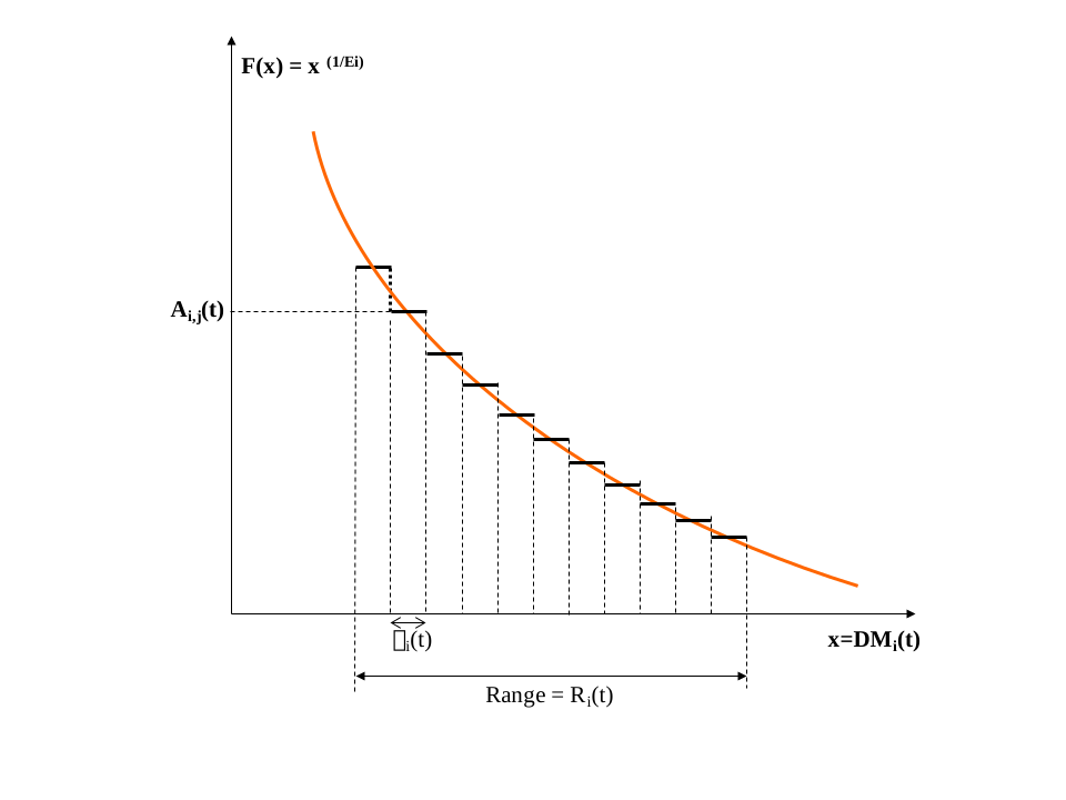
Fig. 4.1 Step-wise constant approximation of the non-linear terms in the objective function.
4.2.4. Calibration of the demand functions
Besides selecting elasticities for the various demand categories, the user must evaluate each constant \(K_i(t)\). To do so, we have seen that one needs to know one point on each demand function in each time period, \(\{p^0_i(t),DM^0_i(t)\}\). To determine such a point, we perform a single preliminary run of the inelastic TIMES model (with exogenous \(DM^0_i(t)\)), and use the resulting shadow prices \(p^0_i(t)\) for all demand constraints, in all time periods for each region.
4.2.5. Computational considerations
Each demand segment that is elastic to its own price requires the definition of as many variables as there are steps in the discrete representation of the demand curve (both upward and down if desired), for each period and region. Each such variable has an upper bound, but is otherwise involved in no new constraint. Therefore, the linear program is augmented by a number of variables, but does not have more constraints than the initial inelastic LP (with the exception of the upper bounds). It is well known that with modern LP codes the number of variables has little or no impact on computational time in Linear Programming, whether the variables are upper bounded or not. Therefore, the inclusion in TIMES of elastic demands has a very minor impact on computational time or on the tractability of the resulting LP. This is an important observation in view of the very large LP’s that result from representing multi-regional and global models in TIMES.
4.2.6. Interpreting TIMES costs, surplus, and prices
It is important to note that, instead of maximizing the net total surplus, TIMES minimizes its negative (plus a constant), obtained by changing the signs in expression (4.5). For this and other reasons, it is inappropriate to pay too much attention to the meaning of the absolute objective function values. Rather, examining the difference between the objective function values of two scenarios is a far more useful exercise. That difference is of course, the negative of the difference between the net total surpluses of the two scenario runs.
Note again that the popular interpretation of shadow prices as the marginal costs of model constraints is inaccurate. Rather, the shadow price of a constraint is, by definition, the incremental value of the objective function per unit of that constraint’s right hand side (RHS). The interpretation is that of an amount of surplus loss per unit of the constraint’s RHS. The difference is subtle but nevertheless important. For instance, the shadow price of the electricity balance constraint is not necessarily the marginal cost of producing electricity. Indeed, when the RHS of the balanced constraint is increased by one unit, one of two things may occur: either the system produces one more unit of electricity, or else the system consumes one unit less of electricity (perhaps by choosing more efficient end-use devices or by reducing an electricity-intensive energy service, etc.) It is therefore correct to speak of shadow prices as the marginal system value of a resource, rather than the marginal cost of procuring that resource.