3. Switches to control the execution of the TIMES code

This Section describes the various GAMS control variables available in TIMES as control switches that can be set by the user in the model <case>.RUN/GEN file for VEDA-FE/ANSWER respectively. As discussed in Section 2, VEDA-FE and ANSWER, in most cases automatically take care of inserting the proper switches into the run file, so the user normally does not have to modify the run file at all. The switches are set in the highly user-friendly GUI interface of the user shell, which uses a run file template and inserts all run-specific switches correctly into the run file of each model run. These are managed by the user via the Case Manager (Control Panel) and Run/Edit GEN Template parts of VEDA-FE and ANSWER respectively.

In the subsections that follow, unless otherwise stated, the basic syntax for the inclusion of control switch options in the main <case>.RUN/GEN GAMS directive file is $SET <option> <value>. The various options are grouped according to the nature of their usage by subsection.

3.1. Run name case identification

The use of the RUN_NAME control variable is practically mandatory when running TIMES. By setting the RUN_NAME control variable, the user gives a name to the model run, which will be used when generating various output files and/or loading information from a previously generated file that has the same name. The control variable is used in the following way:

$SET RUN_NAME runname

Here the runname identifier (corresponding to the run <case> name) is a string of letters, numbers and other characters (excluding spaces), such that the name complies with the rules for the base name of files. It will be used to construct names for the various files comprising a model run, as listed in Table 3.20.

Table 3.20 RUN_NAME TIMES Files

Extension*	Description|
ANT	ANSWER results dump
GDX	GAMS data exchange file (for GAMS2VEDA processing)
*_DP.GDX	Base demand prices to seed a TIMES elastic demand policy run
LOG	Optional GAMS file producing a trace of the model resource usage (activated by lo=1 on the GAMS call line in ANS_GAMS / VT_GAMS.CMD, which needs to be added by the user manually if needed)
LST	GAMS output file with the compile/execute/solve trace, and optional solution dump (via SOLPRINT=YES on the OPTIONS line at the top of the RUN command script)
*_P.GDX	Save/Load point GAMS restart files
RUN	Top level routine calling GAMS (and for VEDA-FE the GDX2VEDA routine)
*_RunSummary.log	Run summary for the associated model run
*_TS.DD	Timeslices declaration for the associated model run
VD*	Suite of results/Set definition(S)/Element description(E)/topology(T) for VEDA-BE

3.2. Controls affecting equilibrium mode

TIMES has a number of variants or model instances embedded in the within the full set of GAMS source code files. Which path through the code is taken is determined mainly the activation (or not) of various control switches, as summarized in this section.

3.2.1. Endogenous elastic demands [TIMESED]

The TIMESED control variable is one of the most important TIMES control variables. It has to be used whenever the full partial equilibrium features of TIMES (that is, employing elastic demands) are to be utilized. For running a baseline scenario to be subsequently used as the reference scenario for partial equilibrium analyses with elastic demands, the following setting should be used:

$SET TIMESED NO

This setting indicates that the user plans to use the resulting price levels from the current run as reference prices in subsequent runs with elastic demands. The setting causes the model generator to create the following (identical) two files from the Baseline run (the second file is a backup copy):

• Com_Bprice.gdx

• %RUN_NAME%_DP.gdx

For running any policy scenarios with elastic demands, using price levels from a previous run as reference prices, one must use the following setting:

$SET TIMESED YES

The reference price levels are read from a file named Com_Bprice.gdx, which is expected to reside in the current directory folder where the model run takes place. Therefore, the Baseline scenario using the setting $SET TIMESED NO has to be run before running the policy scenarios, or the correct Com_Bprice.gdx be otherwise restored from some backup copy.

The VEDA-FE Case Manager (BasePrice) and ANSWER Run (ModelVariant) buttons allow the user to easily control setting of the TIMESED switch and thereby creating/including the Com_Bprice.gdx as appropriate. If neither the base prices are to be written out, nor a policy scenario with elastic demands to be run, the user should not set the TIMESED control variable.

3.2.2. General equilibrium [MACRO]

The general equilibrium mode of TIMES can be activated in two different ways, using the following MACRO control switch settings:

• $SET MACRO YES – activate the standard MACRO formulation

• $SET MACRO MSA – activate the MACRO decomposition formulation

• $SET MACRO MLF – activate the linearized MACRO-MLF formulation

For further information about the standard MACRO formulation, see the TIMES-MACRO documentation available at the ETSAP site.

In all three formulations, the use of the MACRO mode for evaluating policy scenarios requires that so-called demand decoupling factors (DDF) and labor growth rates first have to be calibrated for the Baseline scenario and corre­sponding GDP growth projections. When using the standard MACRO or the Macro-MSA formulation, the calibration produces a file containing the calibrated parameters, which must then be included in the policy scenarios to be evaluated. When using the Macro-MLF formulation, the calibration is done on-the-fly.

Until TIMES v3.3.9, the standard MACRO formulation included a separate utility for calibrating the DDF factors and labor growth rates (see the TIMES-MACRO documentation for details). However, the calibration is much easier using the new MACRO decom­position formulation, where you can use the following MACRO control switch setting for carrying out the Baseline calibration:

$SET MACRO CSA – calibration with the MACRO decomposition method

The “CSA” calibration facility produces a file called MSADDF.DD, which is auto­matically included in any subsequent policy run activated by the MACRO=MSA control switch. In order to carry out the calibration, one must also include the necessary MACRO parameters in the model input data (see the TIMES-MACRO documenta­tion for a description of the MACRO parameters). The only mandatory para­meters are the initial GDP and GDP growth parameters.

The DDF file produced by CSA can be used for the original TIMES-MACRO formulation, where one may re-calibrate it a few times more with the Baseline scenario to verify the calibration for TIMES-MACRO. The re-calib­ration is automatically done by TIMES-MACRO at the end of each run, whereupon a new file DDFNEW.DD is written, which can then be renamed for inclusion in the subsequent TIMES-MACRO policy runs.

When using the Macro-MLF formulation, the Macro equations are calibrated on-the-fly when running any policy scenario. Therefore, no dedicated Macro calibration run is needed for using Macro-MLF, but only a standard Baseline model run is required for obtaining the Base prices, in the same way as when using elastic demands (TIMESED).

When using the MACRO decomposition formulation (with MACRO=MSA or MACRO=CSA), and when the partial equilibrium runs of the Baseline and policy scenarios have already been made, using the LPOINT/RPOINT control settings (in combination with SPOINT) may also be useful (see Section 3.8 and 3.12). If the RPOINT setting is used, the initial solution for the decomposition algorithm is taken directly from the GDX file without having to re-run the previously solved LP model again.

3.3. Controls affecting the objective function

3.3.1. Objective function cost accounting [OBJ]

The user can choose to use several alternative objective function formulations instead of the standard objective function. See Part I, Section 5.3.4 and the documentation for the Objective Function Variants for details. The alternative objective formulations can be activated using the $SET OBJ <option> as described in Table 3.21.

Table 3.21 Objective Function Formulation Options

OBJ Option	Description
ALT	Uses modified capacity transfer coefficients that improve the independency of investment costs on period definitions.
AUTO (default)	TIMES automatically selects the objective function among the standard formulation or the ‘MOD’ alternative formulation according to the B(t) and E(t) parameters specified by the user. If those parameters comply with the assumptions used in the standard formulation, then the standard formulation is used, but if not then the alternative formulation ‘MOD’ is used.
LIN	Assumes linear evolution of flows and activities between Milestone years, but is otherwise similar to the ALT formulation.
MOD	Period boundaries B(t) and E(t) are internally set to be halfway between Milestone years, giving flexibility to set Milestone years to be other than the middle of each period. Investments in Cases I.1.a and I.1.b only of the objective function investment decision are spread somewhat differently across years.
STD	To ensure that the standard formulation is unconditionally used, even if the B(t) and E(t) parameters do not comply with the standard assumptions.

3.3.2. Objective function components

In addition to controlling how the objective function is assembled, as described in the previous section, the user has control of the handling of specific components of the objective functions, as described in Table 3.22.

Table 3.22 Objective Function Component Options

Option <value>	Description
DAMAGE <LP(default)/NLP/NO>	The TIMES model generator supports the inclusion of so-called damage costs in the objective function. By default, if such damage costs have been defined in the model input data, they are also automatically included in the objective function in linearized form (LP). However, if the user wishes the damage costs to be included in the solution reporting only, the DAMAGE control variable can be set to ‘NO’. Non-linear damage functions can be requested by setting the control variable to ‘NLP’. See Part II, Appendix B, for more on the damage cost function extension.
OBJANN <YES>	Used for requesting a period-wise objective formulation, which can be used e.g. together with the MACRO decomposition method for enabling the iterative update of the period-wise discount factors (See the documentation titled Macro MSA, on the MACRO Decomposition Algorithm, for details).
OBLONG <YES/NO>	In the STD (standard) and MOD (alternative) objective function formulations discussed in Table 3.21 the capacity-related costs are not completely synchronized with the corresponding activities, which may cause distortions in the accounting of costs. This switch causes all capacity-related cost to be synchronized with the process activities (which are assumed to have oblong shapes), thereby eliminating also the small problems in salvaging that exist in the STD and MOD formulations. Due to the obvious advantages of using this setting, the OBLONG setting is activated by default whenever the MOD formulation is used. However, for backwards compatibility, one can disable it by adding the explicit setting $SET OBLONG NO in the run file. Using the OBLONG setting can be recommended also with the STD and AUTO settings. It can even be used with the ALT and LIN settings, but that is not recommended.
MIDYEAR <YES>	In the standard objective formulation, both the investment payments and the operating cost payments are assumed to occur at the beginning of each year within the economic/technical lifetime of technologies. This also means that the so-called annuities of investment costs are calculated using the following formula, where r is the discount rate (see Part II, Section 6.2 for more on the objective function): \(CRF = (1-(1+r)^{-1})/(1-(1+r)^{-L})\) According to this formula, the interest costs are zero if the lifetime L of the technology is only one year, because the payments are assumed to occur at the beginning of each year. This approach is often called as beginning-of-year discounting. However, it leads to an underestimation of the costs, because in reality the investments can be paid back only after getting some income from the investment. To avoid such underestimation, the following formula for annuities is perhaps more commonly used: \(CRF = r/(1-(1+r)^{-L})\) This second formula effectively assumes that the annual investment payments occur at the end of each year. This approach is often called as end-of-year discounting. As a good compromise between these two approaches, and highly recommended by many guidelines on good practices in cost evaluations[19], so-called mid-year discounting can additionally be used. See Section 6.2.12 “The discounting methods for annual payments” of Part II for more information about mid-year discounting.
DISCSHIFT	As a generalization to the MID_YEAR setting, alternate time-of-year discounting, including the end-of-year discounting mentioned above, can be achieved by using the DISCSHIFT control variable. The control variable should be set to correspond to the amount of time (in years) by which the discounting of continuous streams of payments should be shifted forward in time, with respect to the beginning of operation. Setting it to the value of 0.5 would be equal to the setting $SET MID_YEAR YES, and setting it to the value of 1.0 would be equal to end-of-year discounting, as follows: $SET DISCSHIFT 1
VARCOST <LIN>	The standard dense interpolation and extrapolation of all cost parameters in TIMES may consume considerable amounts of memory resources in very large models. In particular, the variable costs, which may also be to a large extent levelized onto a number of timeslices, usually account for the largest amount of cost data in the GAMS working memory. If desired, TIMES can be advised to interpolate and extrapolate the variable cost parameters only sparsely for the Milestone years. The values at the intermediate years will then be derived “on the fly”, by piecewise linear interpolation, and will not be stored in the GAMS memory. This option may thus be useful when running very large models on computers with limited memory.

3.4. Stochastic and sensitivity analysis controls

3.4.1. Stochastics [STAGES]

The stochastic mode of TIMES can be activated with the STAGES control variable, by using the following setting:

$SET STAGES YES

This setting is required for using the multi-stage stochastic programming features of TIMES. It can also be used for enabling sensitivity and tradeoff analysis features. See Part I for more details on stochastic programming and tradeoff analysis in TIMES.

3.4.2. Sensitivity [SENSIS]

Many useful sensitivity and tradeoff analysis features are available in TIMES, and they can be enables by activating the stochastic mode of TIMES (see above). However, such sensitivity and tradeoff analyses are often based on running the model in a series of cases that differ from each other in only in a few parameter values. In such cases the so-called warm start features can usually significantly speed up the model solution in the successive runs.

The use of the warm start facilities can be automatically enabled in sensitivity and tradeoff analysis by using the following setting instead of $SET STAGES YES:

$SET SENSIS YES

As the variables then remain the same, warm start is automatically enabled by GAMS according to the BRATIO value (BRATIO can be set in VEDA-FE, or added manually to the ANSWER GEN template as a $OPTION BRATIO=1; as well).

See the documentation on stochastic programming and tradeoff analysis in TIMES for more information on the use of this switch. The documentation is available at the ETSAP site.

3.4.3. Hedging recurring uncertainties [SPINES]

For modeling recurring uncertainties, such as hydrological conditions or fuel-price volatilities, the stochastic mode can be activated also in such a way that the SOW index will be inactive for all capacity-related variables (VAR_NCAP, VAR_CAP, VAR_RCAP, VAR_SCAP, VAR_DRCAP, VAR_DNCAP). This modification to the standard multi-stage stochastic formulation makes it possible to use the stochastic mode for hedging against recurring uncertainties, and for finding the corresponding optimal investment strategy.

This variant of the stochastic mode can be activated by using the following control variable setting:

$SET SPINES YES

In addition, under the SPINES option all the remaining equations that define dynamic or cumulative relationships between variables can additionally be requested to be based on the expected values instead of imposing the inter-period equations separately for each SOW. Doing so will ensure that the uncertainties represented by the SOW-indexed variables will be independent in successive periods. This further model simplification can be requested by using the SOLVEDA switch, as follows:

$SET SOLVEDA 1

In addition, under the SPINES option this SOLVEDA setting will, for now, also cause all the results for the activities and flows to be reported on the basis of the expected values only, and not separately for each SOW. After all, the recurring uncertainties are rather aleatory by nature, and therefore the user should probably be most interested in the optimal investment strategy, and only in the average or normal year results for the activities and flows. If requested, an option to produce results for all SOWs even under the period-independent variant can later be added.

Unlike the basic stochastic option STAGES, the SPINES option may be used also together with the time-stepped mode (see Section 3.5.2).

The SPINES control variable is available only in TIMES versions 3.3.0 and above, and should currently be considered experimental only.

3.5. Controls for time-stepped model solution

3.5.1. Fixing initial periods [FIXBOH]

The purpose of the FIXBOH option is to bind the first years of a model run to the same values determined during a previous optimization. The approach first requires that a reference case be run, and then by using FIXBOH the model generator sets fixed bounds for a subsequent run according to the solution values from the reference case up to the last Milestone year less than or equal to the year specified by the FIXBOH control variable. The FIXBOH control has to be used together with the LPOINT control variable, in the following way:

$SET FIXBOH 2050
$SET LPOINT <run_name>

Here, the value of FIXBOH (2050) specifies the year, up to which the model solution will be fixed to the previous solution, and the value of LPOINT (run_name) specifies the name of the previous run, from which the previous solution is to be retrieved. Consequently, either a full GDX file or a GAMS “point file” (see section 3.8) from the previous run should be available. If no such GDX file is found, a compiler error is issued. The Milestone years of the previous run must match those in the current run.

As a generalization to the basic scheme described above, the user can also request fixing to the previous solution different amounts of first years according to region. The region-specific years up to which the model solution will be fixed can be specified by using the TIMES REG_FIXT(reg) parameter. The FIXBOH control variable is in this case treated as a default value for REG_FIXT.

Example

Assume that you would like to analyze the 15-region ETSAP TIAM model with some shocks after the year 2030, and you are interested in differences in the model solution only in regions that have notable gas or LNG trade with the EU. Therefore, you would like to fix the regions AUS, CAN, CHI, IND, JPN, MEX, ODA and SKO completely to the previous solution, and all other regions to the previous solution up to 2030.

In the RUN file you should specify the control switches described above:

$SET FIXBOH 2030
$SET LPOINT <run_name>

In a model DD file you should include the values for the REG_FIXT parameter:

PARAMETER REG_FIXT
/
AUS 2200, CAN 2200, CHI 2200, IND 2200
JPN 2200, MEX 2200, ODA 2200, SKO 2200
/;

3.5.2. Limit foresight stepwise solving [TIMESTEP]

The purpose of the TIMESTEP option is to run the model in a stepwise manner with increasing model horizon and limited foresight. The TIMESTEP control variable specifies the number of years that should be optimized in each solution step. The total model horizon will be solved by successive steps, so that in each step the periods to be optimized are advanced further in the future, and all periods before them are fixed to the solution of the previous step. Fig. 3.7 illustrates the step-wise solution approach.

Fig. 3.7 Sequence of Optimized Periods in Time-stepped Solution.

The amount of overlapping years between successive steps is by default half of the active step length (the value of TIMESTEP), but it can be controlled by the user by using the TIMES G_OVERLAP parameter. Consequently, the specifi­cations that can be used to control a stepped TIMES solution are the following:

$SET TIMESTEP 20 (specified in the run file)

PARAMETER G_OVERLAP / 10 /; (specified in a DD file)

In this example, the TIMESTEP control variable specifies the active step length of each successive solution step (20 years), and the G_OVERLAP parameter specifies the amount of years, by which the successive steps should overlap (10 years). They may be set in the VEDA-FE Control Panel, like almost all control switches, or in ANSWER by manually adding the parameter to the Run GEN Template.

Because the time periods used in the model may be variable and may not always exactly match with the step-length and overlap, the actual active step-lengths and overlaps may somewhat differ from the values specified. At each step the model generator tries to make a best match between the remaining available periods and the prescribed step length. However, at each step at least one of the previously solved periods is fixed, and at least one remaining new period is taken into the active optimization in the current step.

3.6. TIMES extensions

3.6.1. Major formulation extensions

There are several powerful extensions to the core TIMES code that introduce advanced modeling features. The extension options allow the user to link in additional equations or reporting routines to the standard TIMES code, e.g. the DSC extension for using lumpy investments. The entire information relevant to the extensions is isolated in separate files from the standard TIMES code. These files are identified by their extensions, e.g. *.DSC for lumpy investments or *.CLI for the climate module. The extension mechanism allows the TIMES programmer to add new features to the model generator, and test them, with only minimal hooks provided in the standard TIMES code. It is also possible to have different variants of an equation type, for example of the market share equation, or to choose between different reporting routines, for example adding detailed cost reporting. The extension options currently available in TIMES are summarized in Table 3.23.

VEDA-FE Case Manager and ANSWER Run Model Options form along with the GEN template will both set the appropriate switches and augment the initialization calls, as described in Table 3.23 (unless noted otherwise), with the user being fully responsible to provide the necessary data for each extension option employed in a run.

Table 3.23 TIMES Extension Options

Extension	Description
ABS	Option to use the Ancillary Balancing Services extension. It is activated with the following setting in the <case>.run file: $SET ABS YES See the separate documentation on the ABS extension for more information.
CLI	The climate module estimates change in CO2 concentrations in the atmosphere, the upper ocean including the biosphere and the lower ocean, and calculates the change in radiative forcing and the induced change in global mean surface temperature. It is activated with the following setting in the <case>.run file: $SET CLI YES See Parts I–II for more information on the use of the Climate Module and this switch.
DSC	Option to use lumpy investment formulation. Since the usage of the discrete investment options leads to a Mixed-Integer Programming (MIP) problem, the solve statement in the file solve.mod is automatically altered by the user shell. To activate this extension manually, the following control switch needs to be provided in the <Case>.run file: $SET DSC YES See Part I, Chapter 10 for more information on the use of Lumpy Investment.
DUC	Option to use the discrete unit commitment formulation. To activate this extension manually, the following control switch needs to be provided in the <Case>.run file: $SET DUC YES See separate documentation on Dispatching and unit commitment features in TIMES for more information on the use of the discrete unit commitment option.
ECB	Option to use the Economic Choice Behavior extension (logit market sharing mechanism). To activate this extension, the following control switch needs to be provided in the <Case>.run file, as follows: $SET ECB YES See related user note for more information on the use of this extension.
ETL	Option to use endogenous technology learning formulation. Since the usage of this option leads to a Mixed-Integer Programming (MIP) problem, the solve statement in the file solve.mod is automatically altered by TIMES. To activate this extension manually, the following control switch needs to be provided in the <Case>.run file, as follows: $SET ETL YES See Parts I–II for more information on the use of Endogenous Technology Learning.
MACRO	Option to use the MACRO formulation. Since the usage of the MACRO options leads to a Non-linear Programming (NLP) problem, the solve statement in the file solve.mod has to be altered. To activate this extension manually, the $SET MACRO <value> control switch needs to be provided in the <Case>.run file, with the following valid values: YES – activate the integrated MACRO algorithm MSA – activate Macro decomposition algorithm (MSA) CSA – activate the calibration algorithm for MSA MLF – activate the integrated Macro-MLF formulation See the separate MACRO documentation for more on using these options.
MICRO	Option to use the non-linear elastic demand formulation. To activate this extension manually, the following control switch needs to be provided in the <Case>.run file: $SET MICRO YES See Part II for more information on demand function formulations.
RETIRE	The RETIRE control variable can be used for enabling early and lumpy retirements of process capacities. The valid switch values for this control variable are: NO – Disables all early and lumpy retirements; LP – Enables continuous early retirements for all those processes that are included in the set PRC_RCAP(r,p); MIP – Enables early retirements for the processes that are included in the set PRC_RCAP(r,p), and additionally enables the retirements to be lumpy for those of these processes that also have RCAP_BLK (the lumpy block size) defined, and YES – Enables early retirements for any processes that have at least one instance of the parameter RCAP_BND defined. In this variant, activating lumpy retirements for those processes that have also RCAP_BLK defined requires that the setting $SET DSC YES is used as well. Consequently, when using the $SET RETIRE YES switch, using the set PRC_RCAP is not needed at all (and it will have no effect). See Part II for more information on the use of the Early Retirement feature.
VDA	The VDA control variable can be used to enable the VDA pre-processor extension of TIMES, which implements new features and handles advanced parameters specified by VEDA-FE/ANSWER that are transformed into their equivalent TIMES core parameters to make specification easier (e.g., VDA_FLOP becomes FLO_FUNC/FLO_SUM), with the following setting: $SET VDA YES The VDA extension is always automatically enabled by both VEDA-FE and ANSWER. The attributes implemented are documented in Part II.

3.6.2. User extensions

Besides the core extensions discussed in the previous section, the model management system allows user extensions to be introduced for extended pre-processing of advanced parameter specifications that make the specification of (complex) input parameters much simpler, and to refine features describing technology operations (e.g., for CHPs).

The user extension(s) that are to be included in the current model run need to be activated in the <case>.run file, and passed to inimty.mod, e.g.:

$BATINCLUDE initmty.mod IER FIA

As shown in this example, it is possible to add several extension in the $BATINCLUDE line above at the same time. In this case two user extensions, IER and FIA, are incorporated with the standard TIMES code.

The GAMS source code related to an extension <ext> has to be structured by using the following file structure in order to allow the model generator to recognize the extension[20] (see also Section 2.2). The placeholder <ext> stands for the extension name, e.g. CLI in case of the climate module extension.

• initmty.<ext>: contains the declaration of new sets and parameters, which are only used in the context of the extension;

• init_ext.<ext>: contains the initialization and assignment of default values for the new sets and parameters defined in initmty.<ext>;

• prep_ext.<ext>: contains primarily calls to the inter-/extrapolation routines (prepparm.mod, fillparm.mod);

• pp_prelv.<ext>: contains any preprocessing after inter-/extrapolation but before levelizing;

• ppm_ext.<ext>: contains any preprocessing after levelizing of standard parameters but before calculation of equation coefficients; it might contain calls to levelizing routines for the new input parameters implemented in the extension;

• coef_ext.<ext>: contains coefficient calculations used in the equations or reporting routines of the extension;

• mod_vars.<ext>: contains the declaration of new variables;

• equ_ext.<ext>: contains new equations of the extension;

• mod_ext.<ext>: adds the new defined equations to the model;

• rpt_ext.<ext>: contains new reporting routines.

Not of all these files have to be provided when developing a new extension. If for example no new variables or no new report routines are needed, these files can be omitted.

An example of a user extension is the IER extension included in the TIMES distribution. It contains several extensions to the equation system introduced specifically for the modelling needs by Institute for Energy Economics and the Rational Use of Energy (IER, University of Stuttgart), such as market/product share constraints, and backpressure/condensing mode full load hours.

3.7. The TIMES reduction algorithm

The motivation of the reduction algorithm is to reduce the number of equations and variables generated by the TIMES model, reducing memory usage and solution time. Since there is no downside the having the TIMES reduction algorithm applied by the pre/post-processors, it is the default set via VEDA/ANSWER.

An example for a situation where model size can be reduced is a process with one input and one output flow, where the output flow variable can be replaced by the input variable times the efficiency. Thus the model can be reduced by one variable (output flow variable) and one equation (transformation equation relating input and output flow).

3.7.1. Reduction measures

The effects arising from activating the reduction algorithm are each described below.

1. Process without capacity related parameters does not need capacity variables:

   • No capacity variables VAR_CAP and VAR_NCAP created.

   • No EQL_CAPACT equation created.

2. Primary commodity group consists of only one commodity:

   • Flow variable VAR_FLO of primary commodity is replaced by activity variable.

   • No EQ_ACTFLO equation defining the activity variable created.

3. Exchange process imports/exports only one commodity:

   • Import/Export flow VAR_IRE can be replaced by activity variable (might not be true if exchange process has an efficiency).

   • No EQ_ACTFLO equation defining the activity variable created.

4. Process with one input and one output commodity:

   • One of the two flows has to define the activity variable. The other flow variable can be replaced by the activity variable multiplied/divided by the efficiency.

   • No EQ_PTRANS equation created.

5. An emission flow of a process can be replaced by the sum of the fossil flows multiplied by the corresponding emission factor:

   • No flow variables for the emissions created

   • No EQ_PTRANS equation for the emission factor.

6. Upper/fixed activity bound ACT_BND of zero on a higher timeslice level than the process timeslice level is replaced by activity bounds on the process timeslice level. Thus no EQG/E_ACTBND equation is created.

7. Process with upper/fixed activity bound of zero cannot be used in current period. Hence, all flow variables of this process are forced to zero and need not be generated in the current period. Also EQ_ACTFLO and EQx_CAPACT are not generated. If the output commodities of this process can only be produced by this process, also the processes consuming these commodities are forced to be idle, when no other input fuel alternative exists.

8. When a FLO_FUNC parameter between two commodities is defined and one of these two commodities defines the activity of the process, the other flow variable can be replaced by the activity variable being multiplied/divided by the FLO_FUNC parameter.

   • One flow variable is replaced.

   • No EQ_PTRANS equation for the FLO_FUNC parameter is created.

3.7.2. Implementation

To make use of the reduction algorithm one has to define the environment variable in order to turn on/off the reduction:

$SET REDUCE YES or $SET REDUCE NO

This environment variable controls in each equation where the flow variable occurs whether it should be replaced by some other term or not. If the control variable is not defined at all, the default is to make partial model reduction by eliminating unnecessary capacity variables and substituting emission flows only. This third option can thus be more useful if full model reduction is not wanted.

The possibility of reduction measures is checked in the file pp_reduce.red. If reduction is turned on, flow variables that can be replaced are substituted by a term defined in cal_red.red. The substitution expression for the import/export variable VAR_IRE is directly given in the corresponding equations. In addition the $control statement controlling the generation of the equations EQ_PTRANS, EQ_ACTFLO, EQx_CAPACT has been altered. Also bnd_act.mod has been changed to implement point 6 above.

To recover the solution values of the substituted variables, corresponding parameters are calculated in the reporting routines and are then written to the VEDA-BE file.

3.7.3. Results

The main solution and solver statistics for model runs of a USEPA9r-TIMES model with and without reduction algorithm are given in Table 3.24 for CPLEX (GAMSv24.4.1), using a call to the solver for Barrier for initial solve and Primal Simplex crossover to finish up.

Table 3.24 Reduction Model Comparison

Statistic	Reduce Not Set	Reduce=NO	Reduce=YES
Block / Single Equations	92 / 1,652,677	92 / 1,796,525	92 / 870,814
Block / Single Variables	14 / 2,429,348	14 / 2,564,039	14 / 1,645,631
Total Non-Zeros	7,432,490	8,048,546	5,853,371
Generation	49.499 SECONDS	62.681 SECONDS	45.802 SECONDS
Execution	102.462 SECONDS	115.394 SECONDS	95.972 SECONDS
Memory	2,075 MB	2,180 MB	1,957 MB
Iteration Count	126	116	110
Objective Value	88503425.2162	88151566.0679	88503425.2162
Resource Usage / Solution Time	1323.824	2656.557	1320.111

Comparing the non-setting of REDUCE vs. REDUCE=YES the number of equations and variables in the reduction is around 47% lower than in the non-reduced case. Since the smaller number of equations and variables require less memory, the memory usage in the reduction run decreases by 6.4%. The solution time is only reduced slightly compared to the non-reduced model run.

Issues Using the Reduction Algorithm

• In some cases the reduced problem may produce an “optimal solution with unscaled infeasibilities”.

• Shadow price of non-generated EQ_PTRANS equations are lost.

• Reduced cost of upper/fixed ACT_BND of zero are lost. If one needs this information, one should use a very small number instead, e.g. 1.e-5, as value for the activity bound.

3.8. GAMS savepoint / loadpoint controls

TIMES includes GAMS control variables that can be used to utilize the GAMS savepoint and loadpoint facilities. The savepoint facility makes it possible to save the basis information (levels and dual values of variables and equations) into a GDX file after model solution. The loadpoint facility makes it possible to load previously saved basis information from a GDX file and utilize it for a so-called warm start to speed up model solution.

The GAMS control variables that can be used for the savepoint and loadpoint features in TIMES models are SPOINT and LPOINT. These control variables are completely optional, but can be set in the following ways as described in Table 3.25 if desired:

Table 3.25 Save/Load Restart Switches

Option	Description
SPOINT
Not provided (default)	Does not save or load a restart point.
1 (or YES)	The final solution point from the model run should be saved in the file %RUN_NAME%_p.gdx, where %RUN_NAME% is the GAMS control variable that should always be set to contain the name of the current TIMES model run in the run file for the model.
2	The model generator should make an attempt to load the solution point from the file %RUN_NAME%_p.gdx, where %RUN_NAME% is the GAMS control variable that should always be set to contain the name of the current TIMES model run in the run file for the model. If the control variable LPOINT has additionally been set as well, this attempt will be made only if the loading from the file %LPOINT%_p.gdx fails.
3	Combines both of the functionalities of the settings 1 and 2.
LPOINT
LPOINT filename	Indicates that the model generator should load the solution point from the file %LPOINT%_p.gdx. If the control variable SPOINT has additionally been set to 2 or 3, a subsequent attempt to load from %RUN_NAME%_p.gdx is also made if the loading from the file %LPOINT%_p.gdx fails.

In VEDA-FE the LPOINT can be set from the Case Manager by requesting the loading of a previously GDX, and in ANSWER by means of Run Model Restart files specifications, as shown in Fig. 3.8.

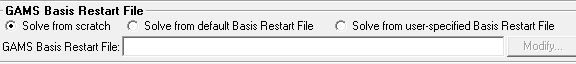
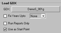
Fig. 3.8 Setting LPOINT

3.9. Debugging controls

By using the DEBUG control, the user can request dumping out all user/system data structures into a file, and turn on extended quality assurance checks. The switch is activated by means of:

$SET DEBUG YES

with actions performed according to the settings described in Table 3.26.

Table 3.26 Debug Switches

Switch <value>	Description
DUMPSOL YES	Dump out selected solution results into a text file (levels and marginals of VAR_NCAP, VAR_CAP, VAR_ACT, VAR_FLO, VAR_IRE, VAR_SIN, VAR_SOUT, VAR_COMPRD, EQG_COMBAL, EQE_COMBAL, EQE_COMPRD).
SOLVE_NOW NO	Only check the input data and compile the source code, but do not solve the model.
XTQA YES	Turn on extended quality assurance checks [this setting is automatically enabled whenever $SET DEBUG YES is used].

3.10. Controls affecting solution reporting

The various $<switch> <value> switches controlling reporting of the model results are summarized in Table 3.27.

Table 3.27 Solution Reporting Switches

Switch <value>	Description
ANNCOST LEV	Until TIMES v3.4.9, the values reported for each of these cost components have been calculated strictly for the associated Milestone year of a period. However this can result in investments made in other years within a period not being reflected, and for longer periods may not properly reflect changes in the other annual expenditures over that timeframe. A consequence of this is that it has not been possible to reconstruct the objective function value from the annualized costs reported. Additionally, these reported costs cannot be thought of as “representative” of the entire period, but only of the Milestone year. To redress this, from TIMES v3.5.0 the annual costs based upon the levelized costs over process lifetimes or periods can be requested. The various annualized cost report parameters are found in Table 3.28. In this way all expenditures during the period are captured and the total objective function can be reconstructed from the levelized annual costs with a very high accuracy (when using $SET OBLONG YES). There is also a new attribute Time_NPV, which gives the period-wise discount factors, and a UC tag = LEVCOST/COST indicating whether the annual costs reported for each scenario are levelized or not. That is, when said Attribute = LEVCOST for a scenario, then the annualized costs for said scenario represent the levelized average annual values.
BENCOST YES	TIMES includes also a basic benefit-cost reporting for new technologies. When the benefit-cost reporting is requested, the TIMES reporting attribute VAR_NCAPR includes the benefit-cost indicators listed in Table 3.29.
RPT_FLOTS COM / ANNUAL	Used for controlling the timeslices that will be used for reporting the levels of the TIMES flow variables. By default, the timeslices of the original TIMES flow variables are used also for reporting. However, in many cases it may be more desirable to have all the flow levels reported at the commodity timeslices (COM), or, for very large models, at the ANNUAL timeslice only. The RPT_FLOTS setting has no effect on the reporting of marginal costs for flows.
SOLANS YES	Produce the solution reports that can be imported into the ANSWER.
SOLVEDA YES / 1	Prepare the solution reporting values that are to be imported into the VEDA-BE. The standard setting is $SET SOLVEDA YES, which works with all TIMES extensions. Sometimes it may be useful to request that TIMES reports also the results from non-stochastic runs with an extra dummy SOW index ‘1’, such that the results can be imported into a database that contains results from both deterministic and stochastic runs. The inclusion of the extra index can be activated by the setting $SET SOLVEDA 1.
XTQA YES	Turn on extended quality assurance checks [this setting is automatically enabled whenever $SET DEBUG YES is used].

Table 3.28 Solution Cost Reporting Attributes

Attribute	Description
Cost_Act	Annual activity costs, plus start-up, shut-down and ramping costs when defined
Cost_Comx	Annual commodity taxes/subsides
Cost_Els	Annual loss of consumer surplus (for elastic demand)
Cost_Flo	Annual flow costs (including import/export prices)
Cost_Flox	Annual flow taxes/subsidies
Cost_Fixx	Annual fixed operating and maintenance taxes/subsidies
Cost_Fom	Annual fixed operating and maintenance costs
Cost_Inv	Annual investment costs
Cost_Invx	Annual investment taxes/subsidies
Cost_ire	Annual implied costs of endogenous trade
Cost_Salv	Salvage values of capacities at EOH+1
Reg_ACost	Regional annual costs by component

Table 3.29 BENCOST Reporting Attributes

Attribute	Description
COST	the total unit costs of VAR_NCAP (in terms of investment costs)
COST	the total unit costs of VAR_NCAP (in terms of investment costs)
CGAP	competitiveness gap (in terms of investment costs), obtained directly from the VAR_NCAP marginals (and optional ranging information)
GGAP	competitiveness gap (in terms of investment costs), obtained by checking also the VAR_ACT, VAR_FLO and VAR_CAP marginals, in case VAR_NCAP happens to be basic at zero
RATIO	benefit / cost ratio, based on CGAP
GRATIO	benefit / cost ratio, based on GGAP
RNGLO	ranging information (LO) for VAR_NCAP (when CPLEX ranging is activated; in terms of investment costs)
RNGUP	ranging information (UP) for VAR_NCAP (when CPLEX ranging is activated; in terms of investment costs)

For the BENCOST report, all of the absolute indicators are expressed in terms of undiscounted investment costs (like those specified by NCAP_COST). For example, the competitiveness gap represents the amount of change in investment costs that would bring the technology competitive (the VAR_NCAP variable would enter the solution basis). Ranging information can only be reported when the CPLEX ranging option has been used. The ranging option can be activated by adding the following two lines into the CPLEX options file (CPLEX.OPT):

objrng VAR_NCAP
rngrestart timesrng.inc

When available, the LO ranging information is also used for calculating the competitiveness gap indicators, because the VAR_NCAP variables can occasionally be basic at zero, making the reduced cost information useless. In such cases the LO ranging value can be used to derive the amount of change required in the VAR_NACP cost coefficient to cause a change in the basis.

3.11. Reporting options activated by RPT_OPT

Various reporting options can also be set by specifying values for the RPT_OPT parameter. Although it is actually not a GAMS control variable, for completeness it is described here. Like the control switches, these options can be specified in the RUN file, but they can also be included in the DD files, if the user shell implements their use that way. Specifying the options in the RUN file can be done with any of the three following alternative ways:

• $SET RPT_OPT KEY1.N1 <value1>, KEY2.N2 <value2>, ...

• PARAMETER RPT_OPT / KEY1.N1 <value1>, KEY2.N2 <value2>, ... /;

• RPT_OPT('KEY1','N1') = <value1>; RPT_OPT('KEY2','N2') = <value2>; ...

Here, KEY1, KEY2, … refer to the main option group and N1, N2, … refer to sub-groups within that group, as indicated in Table 3.30.

Table 3.30 RPT_OPT Options Settings

Option group	Sub-group	Value	Description
ACT	2	<0	Suppress reporting of activity marginals
ACT	9	>0	Filter out process activities less in value than the RPT_OPT value
CAP	9	>0	Filter out process capacities less in value than the RPT_OPT value
FLO	1	>0	Report process flows at commodity TS level
FLO	3	>0	Report value flows by process (implies (FLO,1)=1)
FLO	5	>0	Report electricity supply by energy source
FLO	7	>0	Report process topology indicators
FLO	9	>0	Filter out process flows less in value than the RPT_OPT value (in absolute terms)
COMPRD	1	>0	Report VAR_COMPRD for all commodities
COMPRD	4	>0	Report PRC_MARK constraint marginals in PAR_UCMRK (User_conFXM in VBE)
NCAP	1	<>0	Activate levelised cost calculation (see Part II for details)
NCAP	9	>0	Filter out process new capacities less in value than the RPT_OPT value
OBJ	1	<>0	Split investment costs according to hurdle rate, and report present values of costs by process and commodity (CST_PVP / CST_PVC)
OBJ	2	>0	Report annualized investment costs in terms of costs levelized over the technical life (as with $SET ANNCOST LEV)
COM_TYPE	3	< 0	Report process flows of type COM_TYPE at the ANNUAL level
NRG_TYPE	1	>0	Report the power levels of process flows of NRG subtype NRG_TYPE at COM_TSL level in the P_Out attribute (Var_Pout in VEDA-BE). The value is taken as the conversion factor from the capacity to the flow unit (e.g. 31.536 for PJ/GW).
NRG_TYPE	3	<>0	Report process flows of NRG subtype NRG_TYPE at the ANNUAL level (<0) or at COM_TSL level (> 0, overriding option). With Value=2 one can enable reporting of input flow levels in conjunction with using also sub-group 1.

3.12. Miscellaneous controls

Various other $<option> switches control miscellaneous aspects of a TIMES model run, as described in Table 3.31.

Table 3.31 Miscellaneous Control Options Settings

Option <value>	Description
BOTIME / EOTIME <year>	These controls can be used for adjusting the total available time span of years available in the model. All years related to the data and model must lie between BOTIME and EOTIME, inclusive. The default for BOTIME (‘Beginning of Time’) is 1850 and the default for EOTIME (‘End of Time’) is 2200. [A large model may see slightly faster runtimes if the BO/EOTIME horizon is narrowed to that actually needed for the model run.]
DATAGDX <YES>	This control can be used for requesting all the model input data to be dumped into a GDX file named <RUN_NAME~Data_yymmdd>.GDX, which is saved immediately after all data has been read in, at the beginning of executing the main driver (maindrv.mod). If domain violation warnings have been issued, the GDX file is subsequently used for re-reading the input data with the domain violations filtered. It can also be used for reading all the input data from an existing GDX file in the work folder, which must be then named <RUN_NAME~Data>. In that way, the model data saved from an earlier run can also be used in a new TIMES run, either completely instead of using *.DD data files, or with some new *.DD files merged with the data read from the GDX file. Only the timeslice definition must still be read from a *.DD file.
DYNTS <YES>	This control can be used for enabling dynamic timeslice configurations. Dynamic timeslices means that the timeslice tree can be varied according to model period. See the related user note for more information on the use of dynamic timeslice configurations.
GDX_IREBND / GDX_IPRIC <file>	These control flags can be used to import bounds and prices on exogenous imports/exports from a previous run, and thereby override any user-defined bounds/prices. Only bounds and prices for such imports and exports flows are imported that were endogenous in the previous run but are exogenous for the current run. The first setting tells TIMES to import the flow-levels of imports and exports from the file ‘boundfile.gdx’, and use these levels as fixed bounds on the imports and exports in the current run (if they are exogenous in the current run and were endogenous in the earlier run). The second setting tells TIMES to import the marginal prices of imports and exports from the file ‘pricefile.gdx’, and define these prices on the imports and exports in the current run (if they are exogenous in the current run and were endogenous in the earlier run). The earlier run may have different Milestone years than the current run.
PUNITS <YES>	Used for generating process units info (activity & capacity). The output attribute is PRC_UNITS(r,p,type,units), where type=’ACT’/’CAP’.
RELAX_PRC_CG <YES>	Used to relax the requirement that all genuine commodity groups that are used in process-related attributes have to be explicitly associated with the processes, using the set PRC_CG. All PRC_CG definitions can be omitted in the model when the setting is enabled.
RPOINT <YES>	Used for reproducing the solution of a previous run, without actually solving the model at all. It should be used together with the LPOINT control, which specifies the GDX file where the previous solution is retrieved. The model generator then only loads the solution and generates the reports.
SHELL <ANSWER>	Indicates the ANSWER-TIMES user shell is being used for running this TIMES models.
STSFLX <YES>	Enables the experimental flexible general storage (STS) formulation, which has an enhanced approach for capturing the operational flexibility. See the related user note for more information on this option.
VALIDATE <YES>	A greatly simplified formulation of the objective function and capacity constraints, emulating the MARKAL model generator, may be requested – however, use of the VALIDATE control switch is discouraged.
VAR_UC <YES>	Used to enable or disable the explicit use of slack variables in user constraints. By default, no explicit slack variables are used and all the user constraints are either equalities or inequalities, depending on the bound type specified. However, if the slack variables are enabled, all the user constraints are defined as equality constraints, using bounds on the slack variables to define the actual type of the constraint. This can be useful for e.g. more efficient specification of ranges, and is required when using the stochastic or sensitivity modes.
VINTOPT <1 / 2>	Any technology characteristics defined for a vintaged process describe the characteristics of new capacity installed in the year specified. However, in TIMES the characteristics at the Milestone year are by default used for all the capacity installed in the corresponding period, which can lead to accelerated technology development, depending on the lengths of periods. To avoid such distortions caused merely by period length definitions setting VINTOPT 1 is used, all vintaged characteristics of technologies are automatically adjusted so that the average characteristics of new capacity installed for each period correspond to the original data. When the setting VINTOPT 2 is used, all vintaged processes are modeled using a different approach, which preserves the average characteristics of new capacity installed for each period, as originally defined by the TIMES attributes. The VINTOPT control variable is currently for experimental use only.
WAVER <YES>	Usually the TIMES model generator interpolates the user-defined time-series data only for the Milestone years, and then uses the value at the Milestone year as a representative value for the whole period. An important exception to this common rule are the cost parameters, which are all interpolated densely, and are thus always fully taken into account. However, in some cases it might be desirable to have some other parameters densely interpolated, such that the calculated weighted average over each projection period would be used as the representative value for the period, instead of the value at the Milestone year. Perhaps the most suitable candidates for applying this kind of an interpolation method are parameters representing projected absolute values, such as demands or remaining residual capacities. There is a switch for activating the Weighted Average Interpolation method described above, to be applied for the demand projections (COM_PROJ) and residual capacities (PRC_RESID), as well as the NCAP_PASTI parameters reflecting the available capacity of the installation period.

---

[19]

For example, by the U.S. government: http://www.whitehouse.gov/omb/circulars/a094/a094.html

[20]

This structure is only of interest for those modellers who want to programme their own extensions. The modeller who uses an extension in his model does not need to know these programming details.