3. TIMES DemoS Models
This section explains how to progress in the use of TIMES features and variants using the set of VEDA-TIMES Demo Models. This is a set of VEDA-TIMES models that start from an energy balance and focus on building a model incrementally employing a standard approach to describe the underlying Reference Energy System (RES) as well as specific naming conventions.
The first step model starts with a simple supply curve feeding a single demand. The Demos then grow step by step to build out the RES, adding new commodities, processes (or technologies) and regions, while introducing new attributes (or parameters) and more advanced TIMES modelling features, and explaining the why of the different choices made in VEDA2.0 for building these models.
The VEDA-TIMES Demo Models consist of several incremental steps. Steps 1 to 12 are considered the Basic Demo models (Table 3.32), and are described in this section.). For each step, it provides:
A brief description of the step model and the objectives in terms of VEDA-TIMES features demonstrated;
A summary of attributes introduced and files created, modified, and/or replaced;
A step-by-step description of the template tables created and/or modified in each file; and
A brief look at the results.
Demo |
Folder name |
Short description |
|---|---|---|
001 |
DemoS_001 |
Resource supply |
002 |
DemoS_002 |
More demand options and multiple supply curves |
003 |
DemoS_003 |
Power sector: basics |
004 |
DemoS_004 |
Power sector: sophistication |
005 |
DemoS_005 |
2-region model with endogenous trade: compact approach |
006 |
DemoS_006 |
Multi-region with separate regional templates |
007 |
DemoS_007 |
Adding complexity |
008 |
DemoS_008 |
Split Base-Year (B-Y) templates by sector: demands by sector |
009 |
DemoS_009 |
SubRES sophistication (CHP, district heating) and Trans files |
010 |
DemoS_010 |
Demand projections and elastic demand |
011 |
DemoS_011 |
User SETS in scenario templates |
012 |
DemoS_012 |
More modelling techniques |
3.1. DemoS_001 - Resource supply
Description. This is the first step and therefore represents a very simple model that serves as the starting point for the development of a more complex model: it includes a single supply curve and a single demand for one commodity in a single region over two time periods.
Objective. The objective is to introduce examples of how to implement in VEDA2.0 templates the most basic types of energy commodities and processes that are normally part of a typical TIMES model, along with their respective attributes: a three-step supply curve, an import and an export option, one generic demand and one demand process for one energy commodity (i.e. coal).
This first demo is used also to introduce the SysSettings workbook, the base year template (or VT template), and how to use the most common VEDA2.0 tables.
Attributes Introduced[2] |
Files Created |
|---|---|
G_DYEAR EFF |
SysSettings |
Discount AFA |
VT_REG_PRI_v01 |
YRFR INVCOST |
|
CUM FIXOM |
|
COST LIFE |
|
ACT_BND DEMAND |
|
The first step model is built using only two files: the default SysSettings file and one B-Y Template (VT_REG_PRI_V01). The base year transformation file (BY_Trans) is created by default; it is empty at this stage. Figure 29 shows the VEDA2.0 Navigator (see Section 2.3) for the DemoS_001. This is the first window you will see when you first open it, or switch to it from another model to the DemoS_001. Note that the 1^st^ time you’ll also need to Synchronize the model before proceeding to seed the VEDA2.0 database.
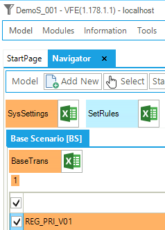
Figure 29. Templates Included in DemoS_001
The RES of this first demo can be viewed in VEDA2.0 (by means of the Item Details see Section 2.5.4), and it is shown in Figure 30. The RES shows an end-use demand device called DTPSCOA, which uses as its input the commodity called COA. The COA commodity can be also exogenously exported outside the model boundary with the export technology called EXPCOA1. The production of the COA commodity is based on one import technology (IMPCOA1) and on a three step local supply curve with the technologies MINCOA1, MINCOA2 and MINCOA3. By double-clicking on any process the RES will cascade to it, then that procedure can be continued by double-clicking on the input/output commodities associated with the process.
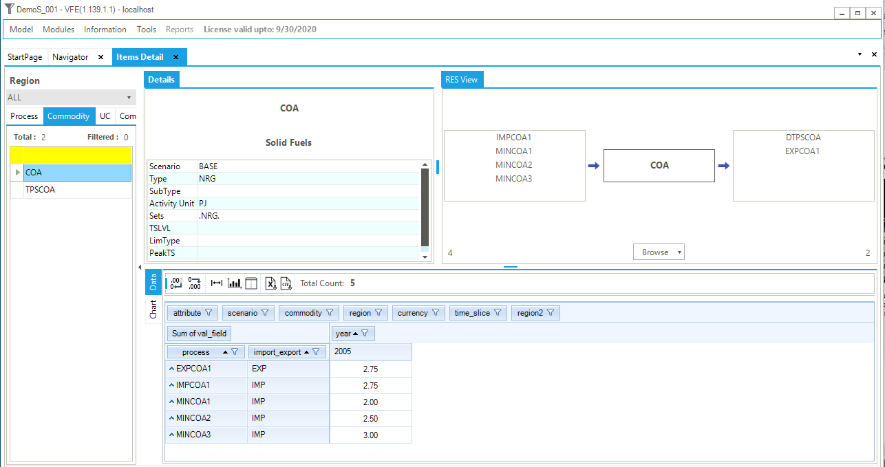
Figure 30. Commodity RES (COA) and Item Details
The next two sections explain VEDA2.0 sheet-by-sheet for the two templates of this first simple DemoS model how this TIMES model for delivering the commodity TPSCOA at the minimum cost is built in VEDA2.0. Note that in the minimal model there is only one region and two files.
3.1.1. SysSetting template
This file is used to declare the very basic structure of any VEDA-TIMES model, including its regions, time slices, start year, etc. It also contains some settings for the synchronization process and can include some additional information. In this example, this file contains the following sheets:
Region-Time slices;
TimePeriods;
Interpol_Extrapol_Defaults;
Constants
Defaults
The key SysSettings Options are shown in Figure 31, and discussed in the sections that follow according to the sheet in the template they are found.
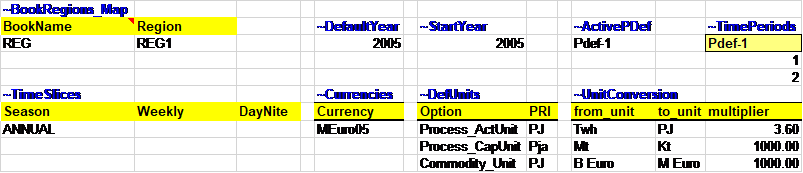
Figure 31. Key SysSettings Options (DemoS_001)
3.1.1.1. Region-Time slices
This sheet contains two tables (see Figure 32):
~BookRegions_Map is used to define:
The workbook name (here, REG), which needs to be the same for each B-Y Template of a region, and
The list of model region names (REG1).
~TimeSlices is used to define the time-slice resolution for the model at different hierarchical levels: SEASON, WEEKLY and DAYNITE. In this first step, there is only one time slice defined by the user for the seasonal level and called ANNUAL.
|
|
|---|
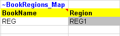
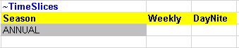
Figure 32. Regions and Time-slices Definition in SysSettings
3.1.1.2. TimePeriods sheet
This sheet contains three tables (Figure 33):
~StartYear is used to define the start year of the model (2005 for this example and all the other steps).
~ActivePDef is used to select the set of active periods (Pdef-1, by default) from all those defined in the following table.
~TimePeriods is used to specify period definitions by specifying the number of years for each period. In this step, only a single period definition has been created (Pdef-1), which contains 1 year for the first period (start year) and 2 years for the second period.
~DefaultYear is used to define the default year of the first period. It default to the StartYear.
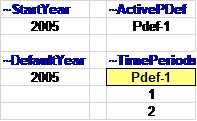
Figure 33. Start Year and Time Period Definition in SysSettings
3.1.1.3. Interpol_Extrapol_Defaults sheet
This sheet normally contains two tables, one for setting user interpolation rules applied to all the other files, unless the user specifies new rules in other templates to overwrite this information, and one for setting the default prices of dummy import processes. There is only the first table in the current version (Figure 34).
~TFM_UPD ACTCOST: is a transformation table used to update pre-existing data in a rule-based manner. In this example, it sets default prices (ACTCOST) for the backstop dummy processes for energy commodities (processes with names matching IMP*Z – dummy IMPort processes ending with “Z”) and demands (IMPDEMZ - a dummy IMPDEMZ process that can feed any demand). These costs should be a few orders of magnitude higher than real import costs in your model in order to ensure that these processes only become active when real fuel supplies are insufficient or unavailable.

Figure 34. Dummy Import Prices in SysSettings
3.1.1.4. Constants sheet
This sheet contains one table (Figure 35):
~TFM_INS global attributes: is a transformation table used to insert new attributes and values in a rule-based manner. In this first step, it is used to declare three new TIMES attributes:
G_DYEAR - discounting year; this is a user input and in this example is 2005;
DISCOUNT - overall discount rate for the energy system, including for depreciation of investments; this is a user input and in this example is 5% and is constant for the entire modelling horizon, and
YRFR - fraction of year for each time slice; this is a user input and in this example is 100% for the single ANNUAL time slice.
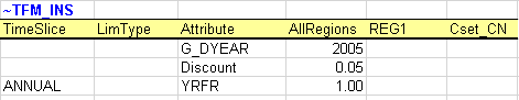
Figure 35. Global Constants Declarations in SysSettings
3.1.1.5. Defaults sheet
This sheet contains two tables shown in Figure 36:
~Currencies: to define a default currency for the whole model; this is a user input. In this example the default unit is million 2005 euros (MEuro05). [It is important to note that for TIMES this is just a label called MEuro05, it is the user’s responsibility to be consistent with costs and units in the model.], and
~DefUnits: to define units for activity, capacity and commodity for each sector in the model: petajoules (PJ) and petajoules per year (Pja) in this case. [Again, it is the user’s responsibility to ensure consistency in the units used in any TIMES model. It is possible to use any units, but it is important to be coherent across the model.].
~UnitConversion: enables unit conversion in the Results module. Use a common unit in to_unit to declare new conversions. For example, for a new energy unit, use PJ in to_unit.
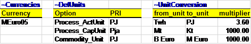
Figure 36. Default Currency and Units Declarations in SysSettings
3.1.2. SysSetting template
This file is used to declare the very basic structure of any VEDA-TIMES model, including its regions, time slices, start year, etc. It also contains some settings for the synchronization process and can include some additional information. In this example, this file contains the following sheets:
Region-Time slices;
TimePeriods;
Interpol_Extrapol_Defaults;
Import Settings (this sheet is not used in the basic DemoS)
Constants
Defaults
Commodity Group. (This sheet is not used in the basic DemoS. In general it can be used to build user commodity groups.)
The key SysSettings Options are shown in Figure 37, and discussed in the sections that follow according to the sheet in the template they are found.
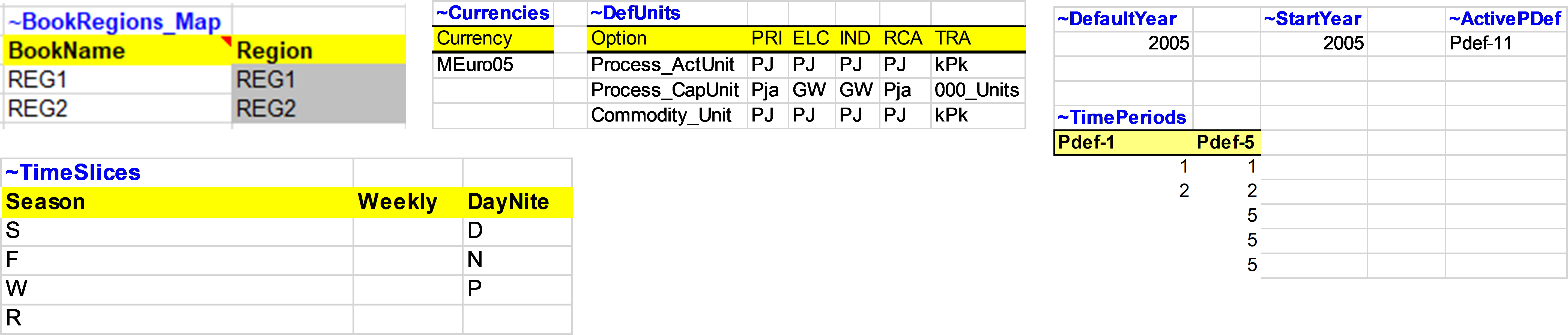
Figure 37. Key SysSettings Options (DemoS_012)
3.1.2.1. Region-Time slices
This sheet contains two tables (see Figure 38):
~BookRegions_Map is used to define:
The workbook name (here, REG), which needs to be the same for each B-Y Template of a region, and
The list of model region names (REG1).
~TimeSlices is used to define the time-slice resolution for the model at different hierarchical levels: SEASON, WEEKLY and DAYNITE. In this first step, there is only one time slice defined by the user for the seasonal level and called ANNUAL.
|
|
|---|
Figure 38. Regions and Time-slices Definition in SysSettings
3.1.2.2. TimePeriods sheet
This sheet contains three tables (Figure 33):
~StartYear is used to define the start year of the model (2005 for this example and all the other steps).
~ActivePDef is used to select the set of active periods (Pdef-1, by default) from all those defined in the following table.
~TimePeriods is used to specify period definitions by specifying the number of years for each period. In this step, only a single period definition has been created (Pdef-1), which contains 1 year for the first period (start year) and 2 years for the second period.
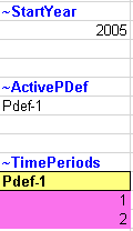
Figure 39. Start Year and Time Period Definition in SysSettings
3.1.2.3. Interpol_Extrapol_Defaults sheet
This sheet normally contains two tables, one for setting user interpolation rules applied to all the other files, unless the user specifies new rules in other templates to overwrite this information, and one for setting the default prices of dummy import processes. There is only the first table in the current version (Figure 34).
~TFM_UPD ACTCOST: is a transformation table used to update pre-existing data in a rule-based manner. In this example, it sets default prices (ACTCOST) for the backstop dummy processes for energy commodities (processes with names matching IMP*Z – dummy IMPort processes ending with “Z”) and demands (IMPDEMZ - a dummy IMPDEMZ process that can feed any demand). These costs should be a few orders of magnitude higher than real import costs in your model in order to ensure that these processes only become active when real fuel supplies are insufficient or unavailable.
Figure 40. Dummy Import Prices in SysSettings
3.1.2.4. Constants sheet
This sheet contains one table (Figure 41):
~TFM_INS global attributes: is a transformation table used to insert new attributes and values in a rule-based manner. In this first step, it is used to declare three new TIMES attributes:
G_DYEAR - discounting year; this is a user input and in this example is 2005;
DISCOUNT - overall discount rate for the energy system, including for depreciation of investments; this is a user input and in this example is 5% and is constant for the entire modelling horizon, and
YRFR - fraction of year for each time slice; this is a user input and in this example is 100% for the single ANNUAL time slice.
Figure 41. Global Constants Declarations in SysSettings
3.1.2.5. Defaults sheet
This sheet contains two tables shown in Figure 42:
~Currencies: to define a default currency for the whole model; this is a user input. In this example the default unit is million 2005 euros (MEuro05). [It is important to note that for TIMES this is just a label called MEuro05, it is the user’s responsibility to be consistent with costs and units in the model.], and
~DefUnits: to define units for activity, capacity and commodity for each sector in the model: petajoules (PJ) and petajoules per year (Pja) in this case. [Again, it is the user’s responsibility to ensure consistency in the units used in any TIMES model. It is possible to use any units, but it is important to be coherent across the model.].
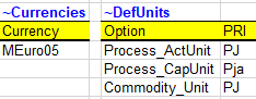
Figure 42. Default Currency and Units Declarations in SysSettings
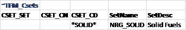
3.1.3. SETS template
The Sets-DemoModels template is used to build user sets (groups) of processes and/or commodities. In this example a commodity set is created (~TFM_Csets) called NRG_SOLID (column SetName) and described as Solid Fuels (column SetDesc). The column Cset_CD (as in any ~TFM table) is used to define the elements that belongs to the set base on the commodity set description so in this example all the commodities that start with any character, SOLID in the middle of the description, and end with any character (* is used as a wildcard).
3.1.4. B-Y Template
The B-Y templates are used to set up the BASE scenario structure of the model, and in principle it is possible to build a full model using just B-Y templates. This is the approach used for this first example. Later when the model grows to include more commodities, technologies, sectors, regions, and additional information to run different scenarios, we will demonstrate the flexibility and modularity of VEDA2.0 using different types of workbooks to input information.
Each B-Y template in the DemoS examples contain worksheets that identify the RES depicted and energy balance used. In this first example the B-Y Template (VT_REG_PRI_V01) is used to set up the base-year process stock and the base-year end-use demand levels, such that the overall energy flows reflect the energy balance.
3.1.4.1. RES&OBJ sheet
This sheet shows the RES covered and the normal completion of a run VEDA2.0with the value of the objective function as reported at the end of the run in VEDA2.0 and the same value in the Results table.
3.1.4.2. EnergyBalance sheet
This sheet contains the energy balance for the model start year (2005) for REG1 (Figure 43). The energy balance in itself is not imported into the model; the table is not identified with any VEDA table header (cell starting with the character “~”). However, it allows the user to calibrate the model start year with appropriate historical energy flows. A typical energy balance comprises two dimensions:
Different types of energy commodities in columns. In this simple example, the different types of energies are partially aggregated in categories (e.g. solid fuels, renewable energies, etc.). The first row of the table includes codes defined by the modeller that are used to name the energy commodities in the model.
Components of the entire supply-demand chain is reflected in rows. This simple example shows three main sections: primary energy supply, energy conversion and final energy consumption. For each energy commodity, the primary energy supply minus the energy used for conversion yield the remainder for final energy consumption. The first column of the table includes codes specified by the modeller that are used to designate the various sectors and then used as part of naming energy processes in a uniform manner in the model.
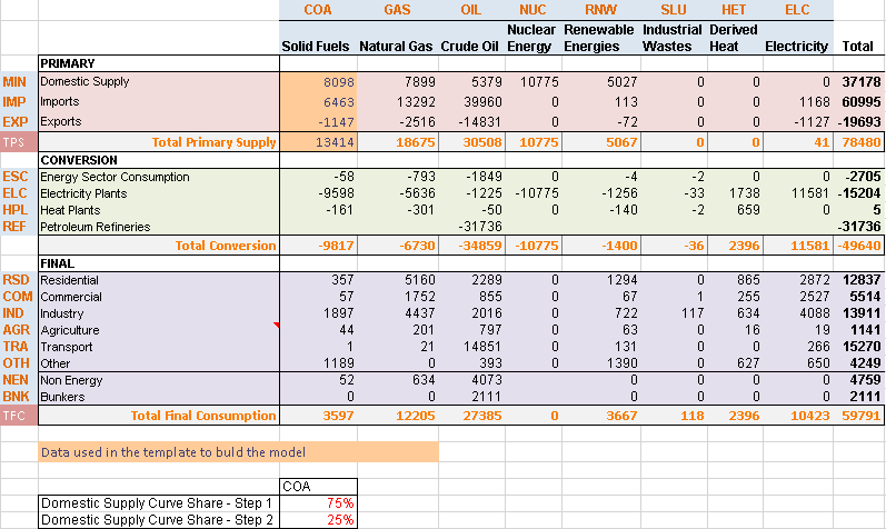
Figure 43. Initial Energy Balance at Start Year (2005) for REG1 in DemoS_001
The portion of the energy balance that is developed in each step model is identified using the color orange: here is this first step primary supply of solid fuels (COA).
Shares are provided below the energy balance table to split the total domestic production of solid fuels (COA) into more than one step. This way, it is possible to set up in the model a supply curve defined by the maximum production and cost of each step. A greater level of disaggregation can be added along both commodity and sector dimensions using additional data sources and user assumptions.
3.1.4.3. Pri_COA
This sheet shows how to declare commodities and processes (in their respective declaration tables) and to describe specific supply processes (in a flexible import table): primary supply of solid fuels (COA) in this example.
In any TIMES model, all commodities and processes in the model need to be declared once in commodity tables (identified with ~FI_Comm) and process tables (identified with ~FI_ Process) with a structure as explained in Sections 2.4.2 and 2.4.3 and shown in Figure 44 and Figure 45.
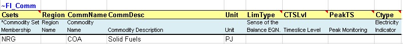
Figure 44. A Typical Commodity Declaration Table
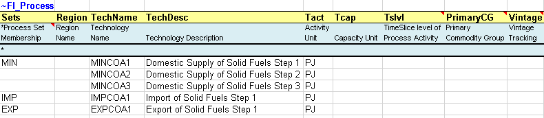
Figure 45. A Typical Process Declaration Table
Unlike the tables used to declare commodities and processes, the tables used to describe specific processes are very flexible (~FI_T). They are built using first Row ID column headers before and below the ~FI_T tag to identify the process names (TechName), descriptions (TechDesc), commodity inputs (Comm-IN), and commodity outputs (Comm-OUT), as well as the years of data (Year) when relevant. Then Data column headers after the ~FI_T are used to provide the data describing the processes. The number and arrangement of rows and columns is totally flexible in these tables. More information about the ~FI_T tables is available in Section 2.4.4.
In the first model step, a flexible import table is used to describe the primary supply options for COA (Figure 46):
A 3-step domestic coal supply curve through three mining processes (MINCOA*), each characterized with the cumulative amount of resources available over the modelling horizon (CUM), the annual cost per unit of energy (COST) and a bound on the annual production (ACT_BND) for the start year 2005 and the following period 2006. Bounds need to be combined with the LimType (UP), which is indicated in a specific column in this example. When not specified, it is UP by default (see Attribute Master Table, Section 2.5.7).
Import and export options are characterized with the COST and ACT_BND attributes.
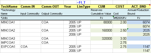
*Blue cells are linked to the energy balance.
Figure 46. Description of Supply Options in a Flexible Table
3.1.4.4. DemTechs_TPS
This sheet shows how to declare commodities and processes (in their respective tables) and to describe specific demand processes (in a flexible import table): a demand process to deliver the total primary supply coal demand, in this example.
A new DEM commodity (TPSCOA -Demand Total Primary Supply – COA) and a new DMD process (DTPSCOA – Demand technology Total Primary Supply – COA) are declared in the commodity and process tables (Figure 47), as described in the previous section.
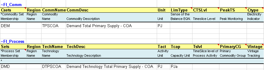
Figure 47. Declaration of Demand Commodity and Process
A flexible import table is used to provide the data depicting the demand option for total solid fuels (Figure 48).
A demand process for the total primary supply of COA (DTPSCOA) is characterized with an efficiency (EFF), an annual availability factor (AFA), an investment cost (INVCOST), a fixed operation and maintenance cost (FIXOM), and a technical lifetime (LIFE). By default this technical lifetime is also used as the economic lifetime, unless a specific economic lifetime (ELIFE) is defined.
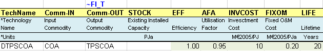
Figure 48. Description of a simple demand processes
3.1.4.5. Demands
This sheet is used to specify the demand (DEMAND) value for the TPSCOA for the base year 2005 (Figure 49). This value comes from the energy balance and represents the total final COA consumption and the total consumed for energy conversion. This demand is constant over the time horizon of the analysis due to the default interpolation/extrapolation applied to the attribute Demand. The future values can be changed by specifying new inputs for the future years/periods.
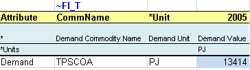
*Blue cells are linked to the energy balance. Here, the demand value is equivalent to the sum of Total Conversion plus Total Final consumption.
Figure 49. Definition of Base Year Demand Values
3.1.5. Solving the Model
The model is solved via the Run Manager (invoked via the StartPage, Modules/RunManager or [F9]), explained more in detail in Section 2.5.5.
For all models of DemoS, all cases (runs) are pre-defined by default (Figure 50) with a name and a description (here, DemoS_001; Demo Step 001), the components to be included in the run (BASE, SysSettings), the Regions (REG1), the Ending Year (2006), and the Period Defs (Pdef-1). It is important to note that the BASE component represents all the base year information included in all B-Y Templates together (only VT_REG_PRI_V01 in this example).
The optimizer options (CPLEX button) and the model variants (Control Panel) are also set by default. The model can be launched by clicking the SOLVE button. The model will be solved using the TIMES source code indicated under GAMS Source Code folder and the results files stored in the folder indicated below GAMS Work folder.
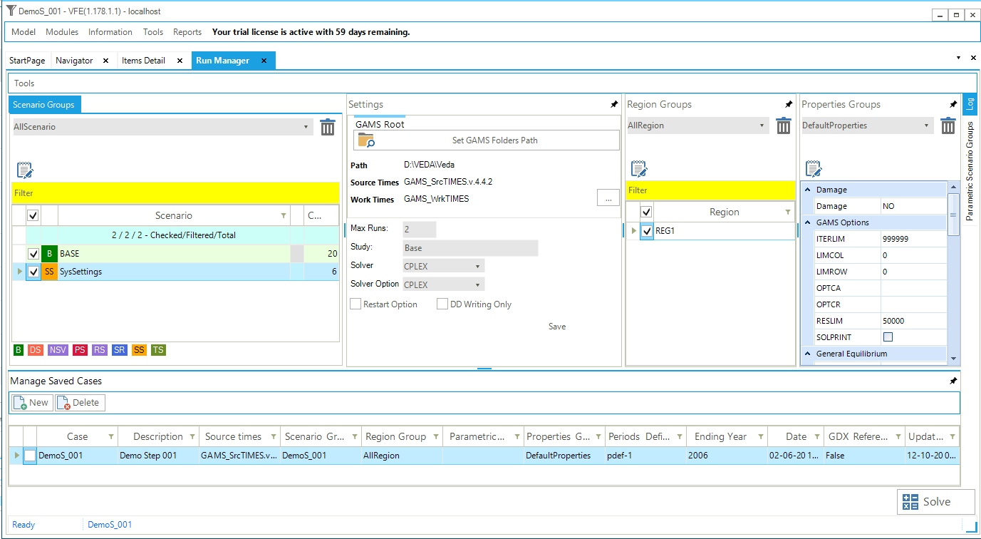
Figure 50. VEDA2.0 Run Manager to Submit Model Runs
3.1.6. Analysis via Results Module
The results of a model run in VEDA2.0 can be imported into the Results manager upon activating it from the StartPage, Modules menus or [f10] key. If the Results form is already open, and new runs submitted, then the  refresh in the upper right can be used to reload the data.
The list of pre-defined tables can be seen by pressing  at the top right of the form. To view a particular table(s), scroll down/up the list and select it (them), then click the Load button. The table will open with a pre-defined layout that can than be modified in a very flexible manner. Not all of the tables can be used for the first demo steps, in which only few results and information will be available. If a Results table is inconsistent or empty you will get a pop up message saying that table is empty.
The Results tables that can be checked for the first DemoS are listed in Figure 51, and then each described below.
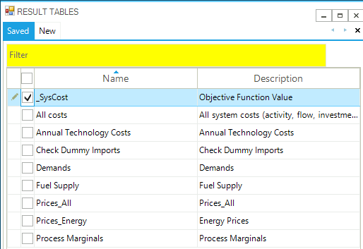
Figure 51. List of DemoS_001 Results Tables
__Check Dummy Imports (Figure 52)
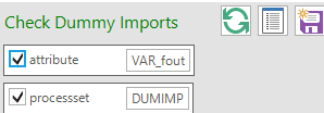
Figure 52. __Check Dummy Imports
In an healthy model this table should be empty. If not, it means the model has some infeasibilities and is using some dummy technologies (built by default in VEDA2.0) to satisfy the commodity/demand production.
This table is built by selecting the attribute VAR_FOUT and the ProcessSet DUMIMP (this is a user-defined process set).
_System Cost Tables
This table (Figure 53), built selecting the attribute Reg_Obj, shows the total system cost discounted to the G_DYEAR defined in the SysSettings file (in this example 2005). Figure 54 shows the total system cost in million euros for the model run to 2006, based on two periods (2005 and 2006) for a total of three years.
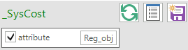
Figure 53. _SysCost Results Table Definition
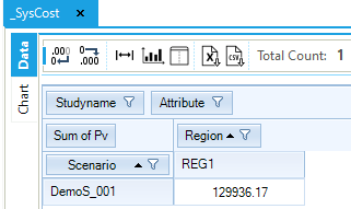
Figure 54. Total System Cost in DemoS_001
The Scenario label shows the scenario name (DemoS_001) for the run we are viewing, while under the column Region we see the region name (REG1) and the value of the objective function. The column Total is shows the total by row (over regions). In this case, we only have the single region REG1, so the value is the same.
The _SysCost table provides a key model run indicator. In TIMES models, the Objective-Function is to minimize the total discounted cost of the system, properly augmented by the ‘cost’ of lost demand (when using the elastic demand features). See Part I and Part II of the TIMES documentation for more on the model objective function.
All costs
This table can be used to show the undiscounted cost elements of the model solution (Figure 55).
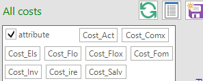
Figure 55. All Costs Results Table Definition
The cost elements, each an individual attribute selected in the table definition, comprise capital costs for investing in and/or dismantling processes (Cost_Inv), fixed O&M costs (Cost_Fom), activity costs (Cost_Act), flow costs including import and export prices (Cost_Flo), implied costs of endogenous trade (Cost_ire), taxes and subsidies (Cost_Flox, Cost_Comx), salvage value of processes and commodities at the end of the planning horizon (Cost_Salv), and welfare loss resulting from reduced end-use demands (Cost_Els).
The undiscounted cost elements (in million euros) that are part of the solution for this first step for REG1 are shown below (Figure 56). [Note that the “fit” button (
 ) was applied once the table was loaded.]
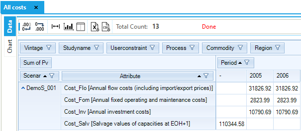
Figure 56. All System Costs Results by Component
The attribute column in this case shows both the attribute name and description, while the Period columns show the value of each attribute in each model period, except the salvage value (Cost_Salv), which does not take a period index.
Demands
The Demands able (Figure 57) is used to show the energy service demand(s). In this case there is only the single demand called TPSCOA, which is in PJ (Figure 58).
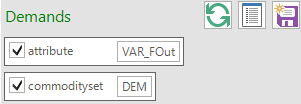
Figure 57. Demands Table Definition
The Demands table shows, from left to right, for the scenario DemoS_001, region REG1, process (or technology) DTPSCOA, a flow out (Var_FOut – production or output from the process) for the commodity Demand Total Primary Supply – COA (TPSCOA), the values for the periods 2005 and 2006.
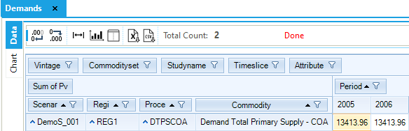
Figure 58. TPSCOA Demand Results Table
Fuel Supply
The Fuel Supply table (Figure 59) is built selecting the attribute VAR_FOut (flow out) and the process set IRE (that includes all the process defined in ~FI_PROCESS tables as MIN, IMP and EXP). In other words, this table can be used to check the output from all the processes that belong to import and mining sets. The export process is characterised with an input and not an output, so it not possible to check the behavior of the export process by selecting only VAR_FOut.
The COA demand is met in a significant proportion with imports (6,462.67 PJ) and the rest with domestic resources through the first two steps of the supply curve. (The third step is not used, because it has higher COST than the imports, see Figure 60.) The demand and supply balance of COA is constant between 2005 and 2006, as described above in Section 3.1.4.5.
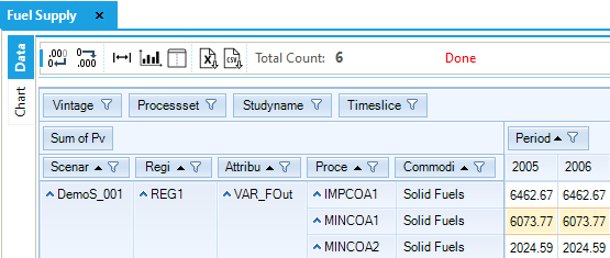
Figure 59. Fuel Supply Results Table
In this example the marginal technology, that is, the technology that would produce the next additional unit of the COA commodity, is the import technology. This information will be reflected in the commodity marginal price for COA, which will be equal to the production cost of the COA commodity from the marginal technology.
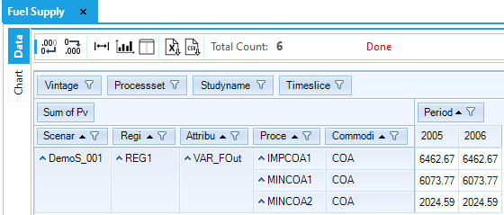
Figure 60. Fuel Supply results by process and period
Prices
The Prices_All table (Figure 61), built selecting the attribute EQ_CombalM, can be used for showing commodities’ marginal prices in the run.

Figure 61. Marginal prices Results Table
As noted above, the marginal price of COA (solid fuels) is the same as the production cost from the marginal technology (import of solid fuels). In this example, it is 2.75 MEuro/PJ in both periods (Figure 62). The marginal price of TPSCOA (Demand Total Primary Supply – COA) in 2005 depends on the new capacity investment that must happen in that year to serve the demand. The marginal price for 2005 can be calculated by taking in account the marginal prices of the solid fuels commodity, the investment cost of the demand technology, the operating cost for the demand technology, and finally the salvage cost. In 2006 there isn’t any new investment, so the marginal price will be only a function of the fuel cost.
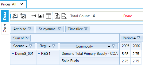
Figure 62. Marginal Prices for DemoS_001 Commodities
3.2. DemoS_002 - More Demand Options and Multiple Supply Curves
Description. The second step model includes a greater number of supply, demand, import and export options for additional commodities in a single region over two time periods.
Objective. The objective is to show how to expand the model with more examples of commodities (energy and emissions) and of typical processes along with their respective attributes, including emission coefficients. On the supply side, it includes more three-step supply curves (e.g., for oil & gas in addition to coal), extraction processes, and import and export options, as well as the introduction of new sector fuel processes (processes used to change fuel names into sectoral commodity names). The demand side is also expanded with the presentation of two demands for energy services (residential and transportation) and corresponding end-use devices in each sector. Emission commodities (e.g. CO2) and emission tracking are also introduced at the end-use device level in both the residential and transport sectors.
Attributes Introduced |
Files Updated |
|---|---|
STOCK |
VT_REG_PRI_v02 |
ENV_ACT |
|
START |
Files. The second step model is built by modifying the B-Y Template (VT_REG_PRI_V02) to add processes as well as energy and emission commodities. The SysSettings file is the same as in the DemoS_001.
3.2.1. B-Y Templates
3.2.1.1. EnergyBalance sheet
The energy balance is the same as in the first step although a larger portion is covered in this second step model (Figure 63). In addition to the primary supply of solid fuels (COA), the model covers the primary supply of natural gas (GAS) and crude oil (OIL) as well as the demand for GAS and OIL in the residential and transportation sectors (rather than for the aggregated primary supply as for COA).
A higher degree of disaggregation is also provided. On the supply side, the same level of disaggregation as for COA is provided for GAS and OIL, with shares to split the total domestic production in more than one step. On the demand side, fuel consumption is split by sector and by end use in the residential sector (space heating, appliances, and other). GAS is allocated at 100% to the Other end use in the residential sector and OIL at 100% to the single end use D1 in the transportation sector.
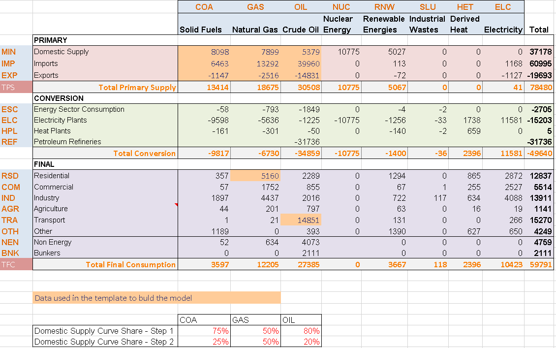
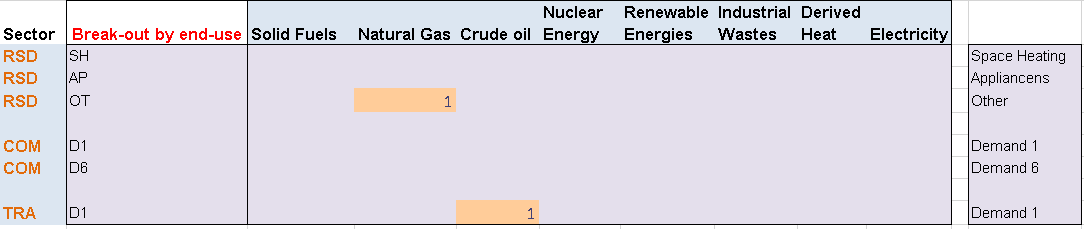
Figure 63. Energy balance at start year 2005 for REG1 – Covered in DemoS_002
3.2.1.2. Pri_COA/GAS/OIL sheets
These new Pri_GAS and the Pri_OIL sheets have exactly the same structure as the Pri_COA sheet (which has not been modified from the first step) including:
A commodity table to declare additional energy commodities (NRG): GAS - Natural gas (PJ) and OIL - Crude oil (PJ).
A process table to declare additional supply options for GAS and OIL: mining processes (MINGAS* and MINOIL*), import processes (IMPGAS1, IMPOIL1), and export processes (EXPGAS1, EXPOIL1).
A flexible import table to describe the primary supply options for GAS and OIL: 3-step domestic supply curves through three mining processes, as well as import and export options. All are characterized with the same attributes.
3.2.1.3. Sector_Fuels sheet
This is a new sheet that is used to construct sector fuel processes (FTE-*), which produce sector fuels from primary fuels, e.g.: GAS becomes RSDGAS and OIL becomes TRAOIL in this example (Figure 64). This is done to make it easy to track fuel consumption at the sectoral level as well as to add sectoral emissions (which could be constrained separately). These technologies can be also used to add additional information on the sectoral commodities, for example additional costs to simulate a sectoral tariff for GAS or an investment cost to simulate new investments in infrastructure and so on. The same approach is used to declare the new commodities and processes in their respective tables.
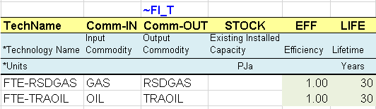
Figure 64. Introduction of Sector Fuel Processes
3.2.1.4. DemTechs_RSD and DemTechs_TRA sheets
Demand processes (DMD) are introduced in these sheets (Figure 65). They consume an energy commodity (RSDGAS, TRAOIL) to produce directly the energy service commodity: residential–other (DROT) and transport (DTD1) in this example. In both sectors, there are existing (ROTEGAS and TOTEOIL) and new processes (ROTNGAS and TOTNOIL).
The existing processes are characterized with their existing installed capacity (STOCK), corresponding in this case to the energy consumption required to produce these energy services in the base year as given by the energy balance and the additional fuel split assumptions. They also have an efficiency (EFF), an annual availability factor (AFA) and a life time (LIFE).
Existing processes characterised in VEDA B-Y Templates with a base year STOCK can not increase their capacity endogenously through new investment because when synchronizing the templates, by default VEDA2.0 inserts the attribute NCAP_BND with interpolation/extrapolation rule number 2, setting an upper bound of EPS (epsilon, or effectively zero) for all years. (For more information on interpolation/extrapolation see Table 3.33 in Section 3.3.2.2) New technologies thus are needed to replace the existing capacity as it retires or increase the amount of capacity available after the base year.
The new processes do not have an existing installed capacity, but they are available in the database to be invested in to replace the existing ones and meet the demand for energy services. They are characterized with an investment cost (INVCOST), a fixed operation and maintenance cost (FIXOM), and the year in which they become available (START). The model can invest in these new technologies only beginning in that START year.
Finally, emission commodities (ENV) are also introduced along with these processes: CO2 emissions in the residential (RSDCO2) and the transport (TRACO2) sectors in this example (in kt). An emission coefficient (ENV_ACT in kt/PJ~output~) is provided for each process based on the technology output. It is also possible to define emissions coefficients based on fuel input (see Section 3.7.2.7).
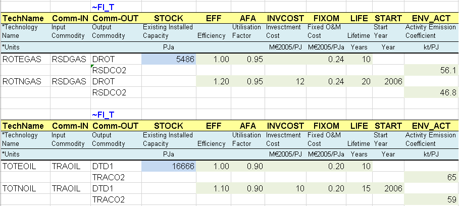
Figure 65. End-use Demand Processes
3.2.1.5. Demands sheet
The demand table is expanded to include the demand for the new energy services created at this step: residential–other (DROT) and transport (DTD1). The 2005 values come from the energy balance sheet and then will be constant, as explained in Section 3.1.4.5, until new data is input for future years.
3.2.2. Results
There are more demands for energy services (Figure 66) and fuel supply options (Figure 67) in this second step model compared with the first step. Also, a new piece of information available at this second step is CO2 emissions by sector (Figure 68), which are computed from the input coefficients provided for each process and the activity of each process. These three tables can be viewed in the same way as explained for DemoS_001, and if results for both DemoS_001 and DemoS_002 have been imported, then it will be possible to see and compare results for the two scenarios. [Note that in order to get the DemoS_001 results into the DemoS_002 database the Tools/Import VD files option must be used to grad them from the GAMS_WrkTIMES subfolder for the model.
The main findings from the results analysis are:
The domestic demand for transportation (DTC1) represents the major proportion (44%) of total domestic demand for energy. This sector relies on oil and also accounts for the largest part of the CO2 emissions (TRACO2), although no coefficient was provided for solid fuels combustion emissions.
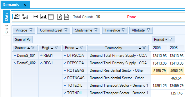
Figure 66. Results - Demands Results Table for DemoS_002
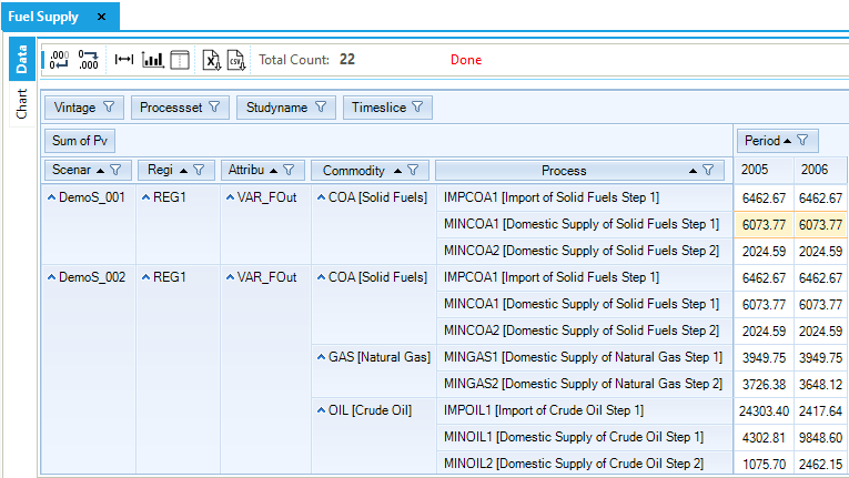
Figure 67. Results – Fuel Supply Results Table for DemoS_002
The demand for residential–other (DROT) and transportation (DTC1) is first fully satisfied with the existing demand processes (ROTEGAS and TOTEOIL) in the base year 2005, but the new demand processes (ROTNGAS and TOTNOIL) start penetrating in 2006. The new processes are more efficient and require less energy to satisfy the demand. The existing processes satisfy less demand in 2006 because their STOCK in 2006 is lower than in 2005. The STOCK decreases between the base year value and zero linearly over the technical LIFE. For example, for ROTEGAS the base (2005) stock is 5486 PJ and will be zero in 2015 (because the residual technical life is 10 years). The stock value between 2005 and 2015 is linearly interpolated between 5486 PJ and 0 PJ.
A large proportion of the oil imported in 2005 is destined to export markets (exports reach their upper limit because the export price is no higher than that of the marginal oil supply, the import price), while in 2006 the demand from export markets decreases to zero and more oil is produced domestically to meet the domestic demand for transportation oil.
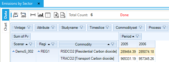
Figure 68. Results – Emissions by Sector Results Table for DemoS_002
Objective-Function = 496 637 M euros (see the _SysCost table).
All the system cost components can be seen from the Results table All costs. As the model includes different types of energy commodities, it is relevant to have a look at their respective marginal prices (Figure 69). Marginal prices of oil are the highest due to higher production costs and import prices. Marginal (shadow) prices for process activity (Figure 70) allow us to understand why the third step of the supply curve for fossil fuels (MINCOA3, MINGAS3, MINOIL3) are not part of the optimal solution, as they are more expensive. For example the VAR_ActM for MINCOA1 is -0.75. This means that if we relax the upper activity bound of this technology of by GJ than the objective function will decrease by 0.75 euros, while forcing the production of 1 GJ from MINCOA3 will increase the objective function by 0.25 euros.
In TIMES, the shadow prices of commodities play a very important diagnostic role. If some shadow price is clearly out of line (i.e., if it seems much too small or too large compared to anticipated market prices), this indicates that the database may contain some errors. For instance, if the shadow price of a commodity is zero and the quantity supplied is non zero, as pointed out by the second theorem of Linear Programming, it means that there is more supply than demand for that commodity. The examination of shadow prices is just as important as the analysis of the quantities produced and consumed of each commodity and of the technological investments.
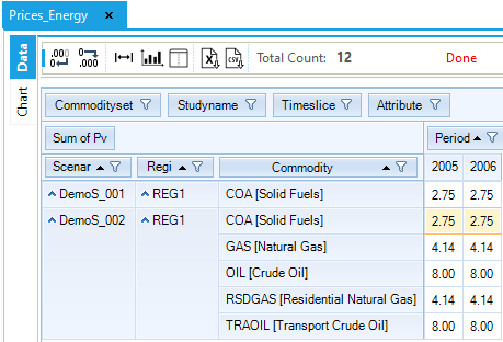
Figure 69. Results – Prices_Energy Results Table for DemoS_002
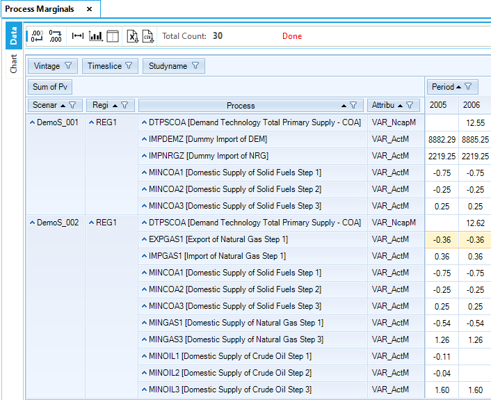
Figure 70. Marginal Price of Process Activity Table in DemoS_002
3.3. DemoS_003 - Power Sector: Basics
Description. The third step model demonstrates the modelling of a simple power sector in a single region over more than two time periods. From the base year of 2005, the time horizon is expanded from 2006 to 2020.
Objective. The objective is to show how to model a typical power sector with different types of power plants (e.g., thermal, nuclear and renewable) along with their respective attributes and the transmission efficiency of the network. Other objectives are to add more time periods, to show how to project future demands (e.g. constant or growing), and to explain the powerful interpolation/extrapolation rules existing in VEDA-TIMES, as well as the difference between model years and data years.
Attributes Introduced |
Files Updated |
|---|---|
COM_IE |
SysSettings |
CAP2ACT |
VT_REG_PRI_v03 |
Files. The third step model is built by modifying:
the SysSettings file to add more time periods and declare the transmission efficiency of the electricity network.
the B-Y Template (VT_REG_PRI_V03) to model the power sector and insert interpolation/extrapolation rules.
3.3.1. SysSettings file
3.3.1.1. TimePeriods sheet
The ~TimePeriods table is used to extend the time horizon of the model by adding three active periods of five years each (Figure 71). These specifications are saved as a new time period definition (Pdef-5). The time horizon is extended to 2020, with the milestones years being 2005, 2006, 2010, 2015 and 2020.
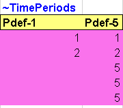
Figure 71. New time periods definition in the SysSettings file
With the introduction of the interpolation/extrapolation rules, it is possible to run the model on a longer time horizon without having to declare data values for all periods up to 2020.
3.3.1.2. Constants sheet
The transformation table is also used to insert a new constant in the model: the transmission efficiency (COM_IE) for the electricity (ELC) commodity in REG1 (Figure 72).
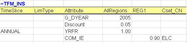
Figure 72. New constant declarations in the SysSettings file
3.3.2. B-Y Templates
3.3.2.1. EnergyBalance sheet
The energy balance is the same as in the second step although a larger portion of it is covered in this third step model (Figure 73). The energy used for conversion into electricity and the total electricity generation are now included.
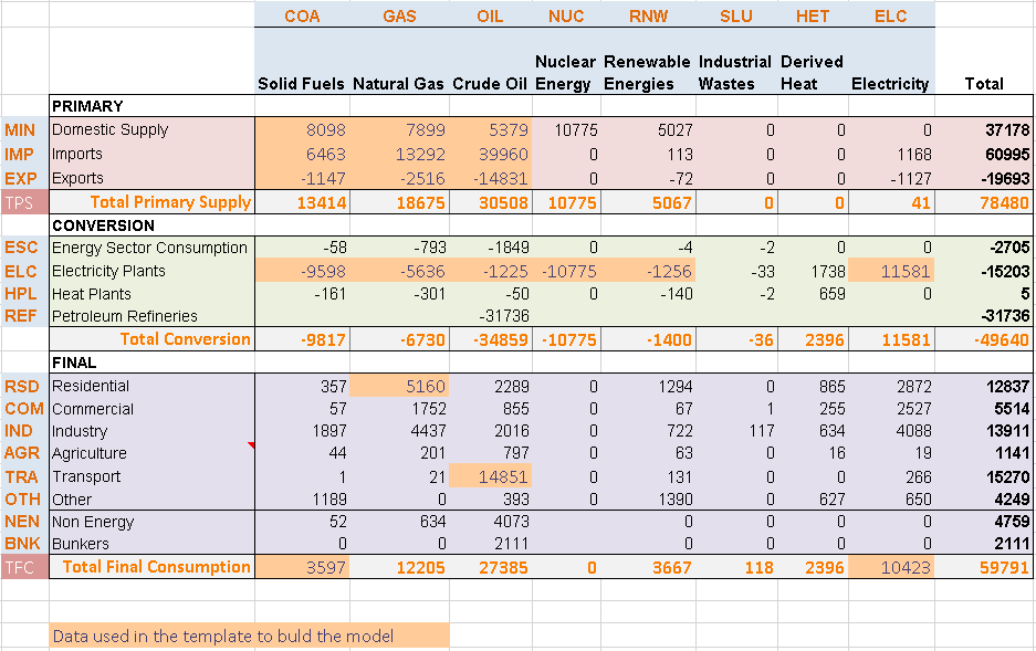
Figure 73. Energy Balance at Start Year (2005) for REG1 – Covered in DemoS_003
3.3.2.2. Pri_COA/GAS/OIL sheets
These sheets were all modified in a similar way to show the use of interpolation/extrapolation rules in VEDA-TIMES (Figure 74). With the introduction of the interpolation/extrapolation rules, it is possible to run the model for a longer time horizon without having to declare data values for all periods up to 2020.
To activate an interpolation/extrapolation (I/E) rule for a specific process, insert a data row and write a “0” as the Year. In this example, an interpolation/extrapolation rule will be enabled for the processes MINCOA1, MONCOA2 and EXPCOA1. Then, an interpolation/extrapolation code is indicated under the attribute. In this example, option 5 will be applied to the activity bound (ACT_BND) of these processes. The option codes for the interpolation/extrapolation rules are presented in Table 3.33. The code 5 means full interpolation and forward extrapolation of the attribute.
In this example, MINCOA1 has an activity bound of 6074 PJ in the year 2005, and due to the I/E rule, the 2005 value is kept constant over the time horizon. Just remember that the ACT_BND is not I/E by default, so when no I/E rule is explicitly specified in the template, the bound will be applied only to the periods defined in the year column.
Default interpolation/extrapolation mechanisms are embedded in the TIMES code itself (for more information see Section 3.1.1 of Part II of the TIMES documentation). It is also useful to check the Attribute Master table in VEDA2.0 (see Section 2.5.7) for more information about which attributes are interpolated/extrapolated by default and which are not.
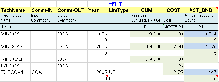
Figure 74. PRI_COA Sheet with Interpolation/Extrapolation Rules
Option code |
Action |
Applies to |
|---|---|---|
0 (or none) |
Interpolation and extrapolation of data in the default way as predefined in TIMES (see below) |
All |
< 0 |
No interpolation or extrapolation of data (only valid for non-cost parameters). |
All |
1 |
Interpolation between data points but no extrapolation. |
All |
2 |
Interpolation between data points entered, and filling-in all points outside the interpolation window with the EPS value. |
All |
3 |
Forced interpolation and both forward and backward extrapolation throughout the time horizon. |
All |
4 |
Interpolation and backward extrapolation |
All |
5 |
Interpolation and forward extrapolation |
All |
10 |
Migrated interpolation/extrapolation within periods |
Bounds, RHS |
11 |
Interpolation migrated at end-points, no extrapolation |
Bounds, RHS |
12 |
Interpolation migrated at ends, extrapolation with EPS |
Bounds, RHS |
14 |
Interpolation migrated at end, backward extrapolation |
Bounds, RHS |
15 |
Interpolation migrated at start, forward extrapolation |
Bounds, RHS |
YEAR (≥ 1000) |
Log-linear interpolation beyond the specified YEAR, and both forward and backward extrapolation outside the interpolation window. |
All |
3.3.2.3. Pri_RNW and Pri_NUC sheets
As with supply curves for fossil fuels, mining processes are created for the uranium resources and the renewable potential (Figure 75). They are considered unlimited and at no cost in this simple example.
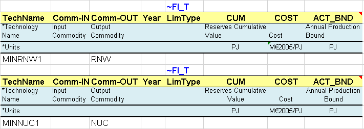
Figure 75. Description of New Supply Options
3.3.2.4. Sector_Fuels sheet
Additional sector fuel processes (FTE-*) are defined and characterized in this sheet, namely to produce the electricity sector fuels from primary fuels, including fossil fuels (e.g. COA to ELCCOA) and other sources (e.g. NUC to ELCNUC). The same approach is used to declare the new commodities and processes in their respective tables.
3.3.2.5. Con_ELC sheet
A series of processes are created to represent different types of power plants (Figure 76). These are conversion processes that consume electricity sector fuels (ELCGAS, ELCNUC, etc.) to produce electricity (ELC).
The existing processes are characterized with their existing installed capacity (STOCK) in GW (calculated from the information given in the energy balance in terms of energy consumption for electricity production and technical attribute values). They also have an efficiency (EFF), an annual availability factor (AFA), fixed and variable O&M costs (FIXOM, VAROM), a life time (LIFE), and a CO2 emission coefficient (ENV_ACT).
By default, all attribute values apply to the base year 2005 when not specified. It is possible to declare any attribute values for future years using the command “~” followed by the year, as for the installed capacity attribute in this case (STOCK~2030). By default, an existing installed capacity (STOCK) decreases to zero at the end of its lifetime (e.g., after 30 years for ELCTECOA00). By specifying an installed capacity value for 2030, as for ELCTENUC00, a new retirement profile is defined (constant in this example), and it is not necessary to specify a life duration.
The new processes do not have an existing installed capacity, but they are available in the database to be invested in to replace the existing ones and meet the demand for electricity. They are characterized in addition with an investment cost (INVCOST) as well as the year where they become available (START).
A new attribute is introduced (CAP2ACT) allowing the conversion between the process capacity and activity units. In this example a coefficient of 31.536 PJ/GW is needed (1GW * 365 days * 24 hours = 8760 GWh = 31.536 PJ). When not specified and when both capacity and activity are tracked in the same unit, the CAP2ACT is equal to 1.
The same approach is used to declare the new commodities and processes in their respective tables (Figure 77) including the declaration of existing and new power plants as ELE processes. The process names follow a convention where T=thermal, C=CHP, R=Renewable, N=Nuclear.
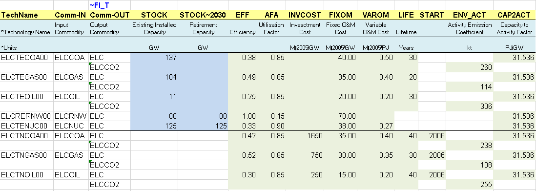
Figure 76. Existing and New Power Plants
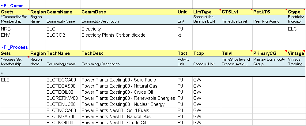
Figure 77. Declaration of Electricity Commodities and Processes
3.3.2.6. DemTechs_ELC sheet
The total demand for electricity (ELC) is modelled in a simplistic manner as for solids fuels (COA). A flexible table is used to describe the demand device for electricity (Figure 78):
A process for the total demand of ELC (DTPSELC) is characterized with an efficiency (EFF), an annual availability factor (AFA), an investment cost (INVCOST) a fixed operation and maintenance cost (FIXOM), and a life time (LIFE).
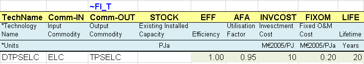
Figure 78. Description of a simple electricity demand processes
3.3.2.7. Demands
The end-use demand table is expanded to include the demand for electricity (TPSELC) in the base year as well as for future years (Figure 79). While the demand for other fuels or for energy services will be kept constant over time (extrapolated at a constant level by default), the demand for electricity is set up to increase by an annual growth rate of 1% through 2020.
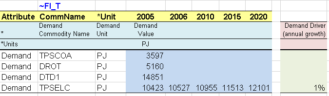
Figure 79. Definition of base year and future years demand values
3.3.3. Results
The demands for energy and energy services are extended to the 2020 horizon (Figure 80), increasing by 1% per year (TPSELC) or remaining constant (all others). The effects of the interpolation/extrapolation rules applied on the activity bound of certain supply processes can be seen below (Figure 63). The activity of the first two mining processes (first two steps of the domestic supply curves) for fossil fuels (COA, GAS, OIL) is controlled by the annual activity bound (set constant for each period by the interpolation rule) and the cumulative bound (CUM). The combination of these two conditions leads to a significant increase in imports to meet the growing demand for energy. Exports are also kept constant using the same interpolation/extrapolation rules. More primary supply options exist now with the addition of the electric fuels such as nuclear and renewables.
Results from the new electricity sector are introduced (Figure 82 and Figure 83). The total generating installed capacity increases from 466.3 GW in 2005 to 541.6 GW in 2020. Most of this increase is coming from new coal-fired power plants (ELCTNCOA00), the most expensive process but the least expensive fuel. The installed capacity of nuclear and renewable power plants remain constant as specified in the B-Y Template. Electricity production is coming mainly from fossil fuels (64%), with a smaller contribution from nuclear (26%) and renewables (9%). The oil plants are working only in the base year, as calibrated to the energy balance, because the fuel is too expensive compared to the other available options.
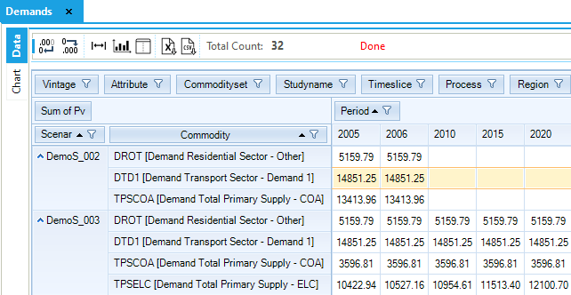
Figure 80. Demand Results Table in DemoS_003
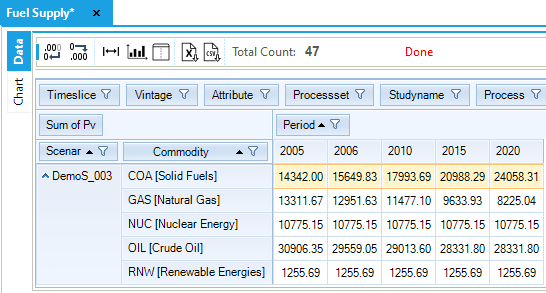
Figure 81. Fuel Supply Results Table in DemoS_003
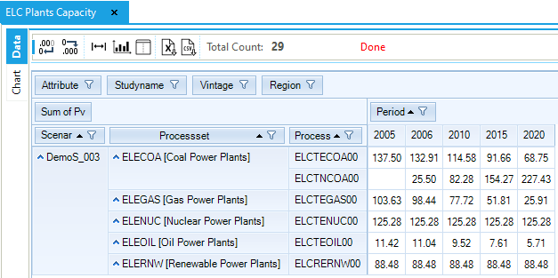
Figure 82. Electricity Plants Capacity Results Table in DemoS_003
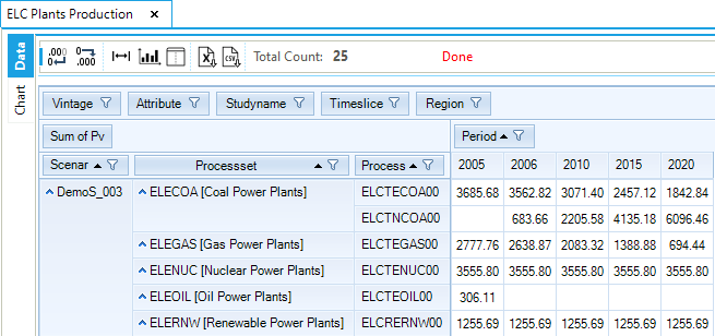
Figure 83. Electricity Plants Activity Results Table in DemoS_003
Objective-Function = 3,185,019 M euros (see the _SysCost table). This cost is significantly higher compared to the optimal cost obtained with DemoS_002 because of the addition of the electricity sector. All the system cost components can be seen in the Results table All costs, as well as the marginal fuel prices in Price_Energy and the process activity in Process Marginals.
3.4. DemoS_004 - Power sector: sophistication
Description. The fourth step model expands the modelling to a more sophisticated power sector in the same single region over the 2020 horizon.
Objective. The objective is to introduce the concepts of time slices, peak, and peak reserve capacity. Time slices are added to the model to adequately capture the timing of the electricity demand, and the peak reserve capacity requirement is illustrated through scenario variants, with and without peak reserve capacity factor. This step model is also used to show how interpolation/extrapolation specifications can be moved to the SysSettings file and applied to all instances of an attribute in the model using a single declaration.
Attributes Introduced |
Files Updated |
|---|---|
PEAK |
SysSettings |
COM_FR |
VT_REG_PRI_v04 |
Discount |
Files Created |
COM_PEAK |
Scen_Peak_RSV |
COM_PKRSV |
Scen_Peak_RSV-FLX |
COM_PKFLX |
Files. The forth step model is built:
by modifying the SysSettings file to add new time slices and to insert default interpolation/extrapolation options;
by modifying the B-Y Template (VT_REG_PRI_V04) to declare the contribution of power plants to the peak and add the load curve of electricity demand;
by creating scenario files to illustrate the peak reserve capacity requirement (Figure 84).
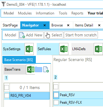
Figure 84. Templates In DemoS_004
3.4.1. SysSettings file
3.4.1.1. Region-Time Slices
The ~TimeSlices table is used to create four time slices (Figure 85) and replace the previous single ANNUAL time slice. There are four time slices combining two seasons (W- Winter and S- Summer) and two intraday periods or day-night periods (D- Day and N- Night).
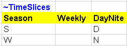
Figure 85. New Time Slices Definition in SysSettings
3.4.1.2. Interpol_Extrapol_Defaults
A table is added for setting the default interpolation/extrapolation rules (
Figure 86). A transformation table used to update pre-existing data (~TFM_MIG) in a rule-based manner, it sets the default interpolation/extrapolation rule, indicated by the 0 in the Year2 column, for the attribute defined in the Attribute column and all the processes defined in the model. In this case, this is the same interpolation/extrapolation rule used for each of the supply processes (see Figure 30) in the B-Y Template. It is now moved into the SysSettings file and applied to the activity bound (ACT_BND) of all processes at once.
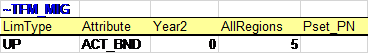
Figure 86. Default Table for Interpolation/Extrapolation Rules in SysSettings
3.4.1.3. Constants
The existing transformation table is also used to insert new constants in the model: fractions of year for the new time slices (YRFR) replace the single ANNUAL time slice (100%) as declared in the previous steps (Figure 87). The timeslice name is identified in the first column (TimeSlice), while their fractions (for the attribute called YRFR) over one year are declared for AllRegions as for the other constants of the model. The fraction values, as with any other input in the model, are the user’s responsibility. In this case, it is important that they sum to 100%.
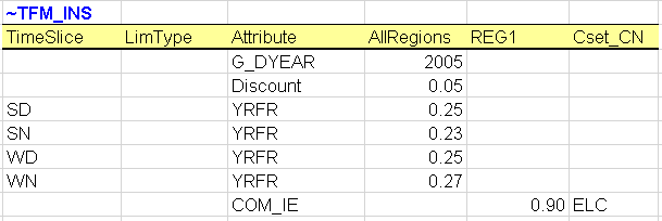
Figure 87. New Time Slice Declarations in SysSettings
3.4.2. B-Y Templates
3.4.2.1. Con_ELC
A new attribute is declared for all existing and new processes representing power plants (Figure 88):
Their contribution to peak (Peak), i.e., the fraction of a process’s capacity that is considered to be secure and thus will most likely be available to contribute to the peak (and reserve capacity) load in the highest demand time-slice of a year for a commodity (electricity or heat only). In this case, the capacity contribution of all thermal and nuclear power plants is 100%, while the capacity contribution of the renewable power plant is 50%. Indeed, many types of supply processes can be regarded as predictably available with their entire capacity contributing during the peak and thus have a peak coefficient equal to 1 (100%), whereas others (such as wind turbines or solar plants) are attributed a peak coefficient less than 1 (100%), since they are on average only fractionally available at peak. (E.g., a wind turbine typically has a peak coefficient of 0.25 or 0.3 maximum).
Another important change to mention is the start year of one new process (ELCTNOIL00) that can be installed from the 2005 base year to cover the additional capacity needed for the reserve equation (5%), as defined in the scenario files.
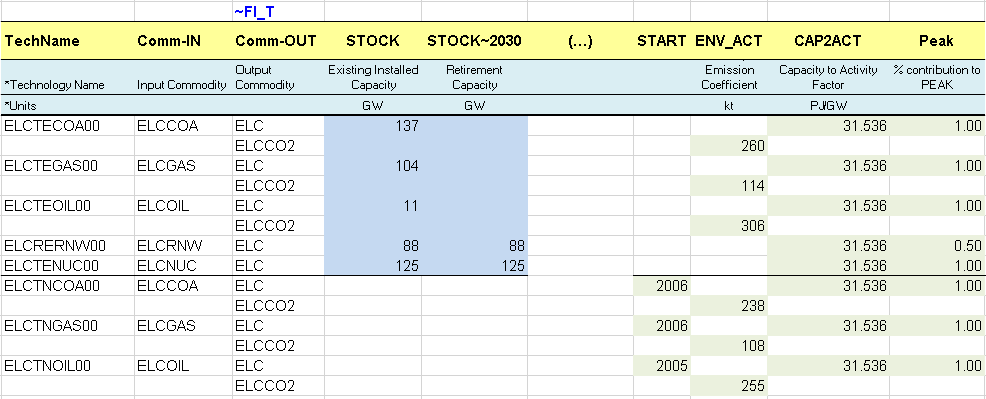
Figure 88. Peak Contribution for Different Types of Power Plants
Additional information is required to complete the declaration of the electricity commodity and processes in their respective tables (Figure 89 and Figure 90). Along with the new time slices, it is possible to specify the tracking level of the electricity commodity (ELC) in the CTSLvl column: DAYNITE. (When not specified, as in the previous step, the default is ANNUAL.) PeakTS (peak time slice monitoring) directs TIMES to generate the peak equation for the specified time slices. It is possible to declare any of the time slices defined in the SysSettings file, or ANNUAL (the default) to generate the peaking equation for all time slices. Since it is left blank here, the peak equation will be generated in all time slices once it has been requested using COM_Peak (see Section 3.4.3.1). Finally, it is important that the user enter ELC in the Ctype column when declaring an electricity commodity that may be produced by combined heat and power (CHP) plants, as this commodity will be in DemoS_009.
For the electricity processes, the process table is used to define the time slice level of operation in the Tslvl column (Figure 90). For example, the coal-fired and the nuclear power plants are defined at the SEASON time slice level, meaning that their operational level does not vary across DAYNITE time slices. (When not specified, the default is based on the Sets declaration: DAYNITE (for ELE), SEASON (for CHP and HPL) ANNUAL (for all others).)
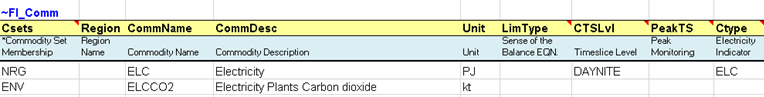
Figure 89. Declaration of Time Slice Level for Electricity Commodity
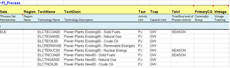
Figure 90. Declaration of Time Slice Operational Level for Processes
3.4.2.2. Pri_COA/GAS/OIL
These sheets were all modified back to remove the interpolation/extrapolation rules: the flag to activate an interpolation/extrapolation rule (additional rows with a “0” as the Year) and the rule code in the attribute column.
3.4.2.3. Demands
A table is added to define the load curve of the demand for electricity (TPSELC) in the base year, which will also apply for future years (Figure 91). The attribute (COM_FR) is introduced to declare the fraction of the electricity demand occurring in each time slice.
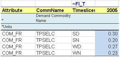
Figure 91. Definition of Load Curve for Electricity Demand
The TPSELC commodity is the demand commodity produced by a demand technology (end-use technology) called DTPSELC (Figure 92) and defined in the sheet DemTechs_ELC. This technology takes as input the ELC commodity that will be consumed by timeslice as defined by the COM_FR attribute for TPSELC.
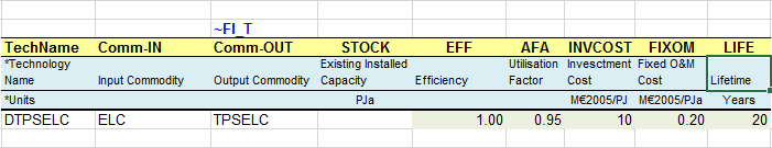
Figure 92. Demand Technology Producing TPSELC
3.4.3. Scenario files
3.4.3.1. Scen_Peak_RSV and Scen_Peak_RSV-FLX
Two scenario files are created to insert new information in the RES that can be retained or not in the configuration of the model at the time of solving the model (see Section 2.5.5). A transformation table ~TFM_INS is used to declare new attributes (Figure 93):
COM_Peak - Specify that the peaking equation will be generated for the ELC commodity.
COM_PKRSV - Declare the capacity fraction (%) that is required for the peak reserve. This is the option used in the first scenario file (Peak_RSV).
COM_PKFLX - Declare the fraction (%) by which the actual peak demand exceeds the average calculated demand, by time slice. This is the option used in the second scenario file (Peak_RSV- FLX) for the Summer-Day time slice (SD), although in practice COM_PKFLX is typically used alongside COM_PKRSV.
The TIMES peak equation allows the user to require that the total capacity of all processes producing a commodity at each time period and in each region exceed, by a certain percentage, the average demand in the time-slice when the highest demand occurs. This peak reserve factor (COM_PKRSV) insures against several contingencies, such as possible commodity shortfall due to uncertainty regarding its supply (e.g. water availability in a reservoir), unplanned equipment down time, and random peak demand that exceeds the average demand during the time-slice when the peak occurs. This constraint is therefore akin to a safety margin to protect against random events not explicitly represented in the model. Optionally, COM_PKFLX can be used to reflect the fact that the actual system peak demand is greater than the average demand in the model’s peak slice, allowing COM_PKRSV to represent a more typical utility reserve margin.

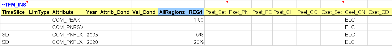
Figure 93. Declaration of the Peak Reserve in a Scenario File
3.4.4. Results
Three cases are solved with this step model, with a different selection of scenario files (Figure 94): the DemoS_004 case is solved using only the two components (BASE, SysSettings), while the DemoS_004a case is solved adding one scenario file (Peak_RSV), and the DemoS_004b case is solved adding the other scenario file (Peak_RSV-FLX). The different Cases in the Run Manager can be selected individually to run a single Case or multiple Cases selected to be submitted in parallel (i.e., the cases will be launched automatically by VEDA2.0 one after the other) to TIMES.
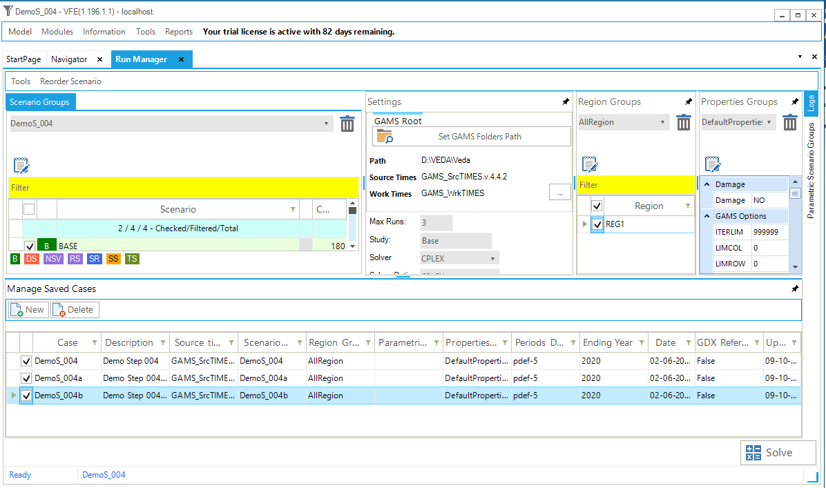
Figure 94. Solving Multiple Cases
The impacts of the improvements made in the electricity sector on the electricity generating capacity are shown in Figure 95, namely.
The effect of adding new time slices and of specifying the seasonal operational level for the coal-fired power plant in DemoS_004, compared with DemoS_003: there is a switch from coal-fired generation to natural gas-fired generation due to its greater flexibility (time slice level DAYNITE for gas, as opposed to SEASON for coal) to satisfy the electricity demand. The additional natural gas supply is coming from import sources.
The effect of declaring a peak reserve factor on the total capacity in DemoS_004a, compared with DemoS_004: there is additional capacity required that is coming from oil-fired power plants as new power plants are available from 2005. The total capacity in DemoS_004a is increasing from 507 GW in 2005 to 659 GW in 2020 (compared with 466 GW to 542 GW without the peak reserve requirement).
There is no effect on the generating capacity in DemoS_004b, compared with DemoS_004a.
The electricity price varies across years and time slices (Figure 96).
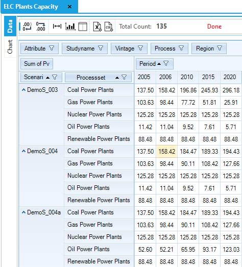
Figure 95. Electricity Plant Capacity Results Table in DemoS_004
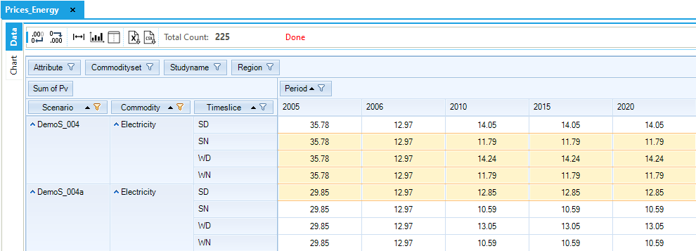
Figure 96. Electricity Price by Time Slice in DemoS_004
Other interesting results to show are related to the peak contribution specifically (Figure 97). The peak equation expresses that the available capacity must exceed demand for the electricity (ELC) commodity in any time slice by a certain margin, so the dual value of the peak equation describes the premium consumers have to pay in addition to the commodity price (dual value of EQ_COMBAL) during the peak time slice (SD in this case) to ensure adequate system capacity. The peak marginal is similar, though not identical, when using COM_PKRSV and COM_PKFLX, owing to the differences in how they are applied in the TIMES equations.
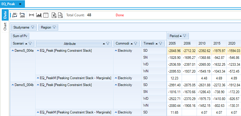
Figure 97. Slack and Dual Values of the Peak Equations in DemoS_004
Objective-Function = 3,187,361 M euros (see the _SysCost table). This cost is only slightly higher with the peak reserve requirement and the additional investments in generating capacity: 3,211,296 M euros.
3.5. DemoS_005 - 2-region Model with Endogenous Trade (compact approach)
Description. At the fifth step, the model evolves from being a single region model to become a compact multi-regional model (2 or more regions in the same set of B-Y Templates). This approach is relevant when all the model regions are under the control of a single individual.
Objective. The objective is to create the multi-regional model framework typical to larger or more complex models, namely the trade matrix that allows the modelling of energy trade movements (uni-directional or bi-directional trade between two regions). Another objective is to demonstrate how to limit emissions from a sector in a particular region or from the entire energy system of all regions through emission bounds or user constraints. Scenario variants illustrate the impact of a cap on CO2 emissions from the electricity sector only and of a cross-region user constraint on the total CO2 emissions from the transport and electricity sectors.
Attributes Introduced |
Files Updated |
|---|---|
COM_BNDNET |
SysSettings |
UC_RHSRTS |
VT_REG_PRI_v05 |
UC_COMNET |
Files Created |
Scen_TRADE_PARAM |
|
Scen_ELC_CO2_BOUND |
|
Scen_UC_CO2BND |
|
Files Removed |
|
Scen_Peak_RSV-FLX |
Files. The fifth step model is built:
by modifying the SysSettings file to add one region;
by modifying the B-Y Template (VT_REG_PRI_V05) to disaggregate the energy balance between two regions and to regionalize some process attributes;
by creating trade files to capture the trade movements between the two regions;
by creating more scenario files to limit GHG emissions (Figure 98).
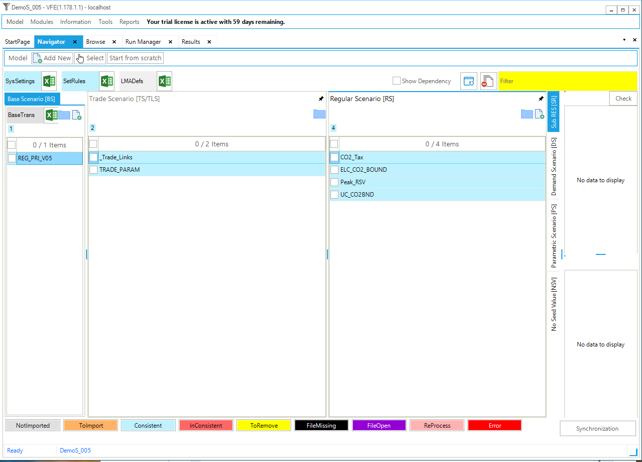
Figure 98. Templates In DemoS_005
3.5.1. SysSettings file
3.5.1.1. Region-Time Slices
The ~BookRegions_Map table is used to create one additional region: REG2 (Figure 99) in the same workbook (REG).
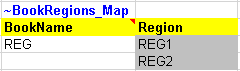
Figure 99. New Region Definition in SysSettings for DemoS_005
3.5.2. B-Y Templates
3.5.2.1. EnergyBalance, EB1, EB2
The energy balance is disaggregated between two regions (Figure 100) using shares on production, conversion, and final consumption of various energy commodities: REG1 becomes producer and consumer of solid fuels (100%), crude oil (30%) and renewable energies (100%), while REG2 becomes producer and consumer of natural gas (100%), crude oil (70%), and nuclear energy (100%). The same portion of the energy balance as in the fourth step is used in this fifth step model.
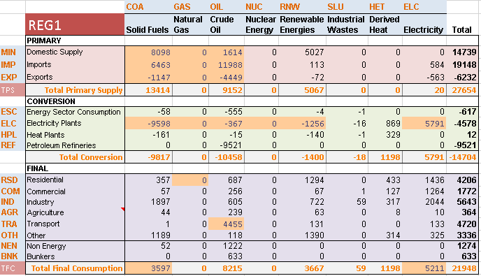
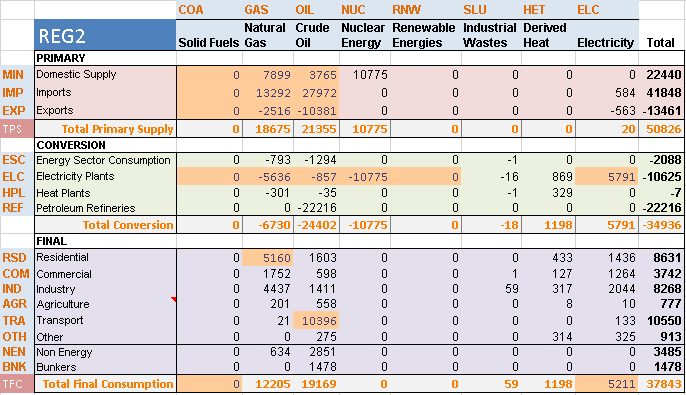
Figure 100. Energy balance at start year 2005 for REG1 & REG 2–Covered in DemoS_005
3.5.2.2. Pri_COA/GAS/OIL
These sheets are updated to include two regions and to regionalize some process attributes. There are several ways of accounting for the regionalization of some attributes. For instance, it is possible to insert a Region column on the left side of any ~FI_T table and to indicate in which region(s) the process is available (Figure 101). A process can be available in only one region (e.g. MINGAS* and IMPGAS1) or in several regions (EXPGAS1). In this later case, different rows can be inserted to declare different values for some of the attributes (ACT_BND of EXPGAS1); the values that remain on the initial row will apply to all regions (COST of EXPGAS1). The additional rows approach is mainly used when all attributes of a process vary across regions.
In the process table (~FI_ Process), the region where each process is available can be specified (Figure 102): MINGAS* and IMPGAS1 processes exist only in REG2, while the EXPGAS1 process exists in both regions (by default, when the Region column is empty, it applies to all regions). Comma-separated entries are also allowed, for instance, when a process exists in more than one region but not in all regions.
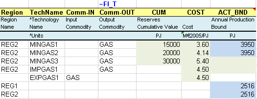
Figure 101. Regionalization of Process Attributes using Additional Rows
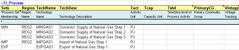
Figure 102. Region Specification in the Default Process Table
3.5.2.3. Con_ELC
This sheet is also updated to include two regions and to regionalize some process attributes. However, a different approach is used (Figure 103): columns are inserted (duplicated) only for those attributes that vary across regions: the STOCK attribute in this example. As for the year, the regions are identified using the “ ~ “ command after the attribute. The additional columns approach is mainly used when only few attributes of a process vary across regions.
The column approach is also used in the following sheets, namely for the STOCK attribute: Sector_Fuels, DemTechs_TPS, DemTechs_ELC, DemTechs_RSD and DemTechs_TRA. The row approach is used in the Demand sheet.
3.5.3. Trade files
Two trade files are created to model the energy trade movements between the two regions.
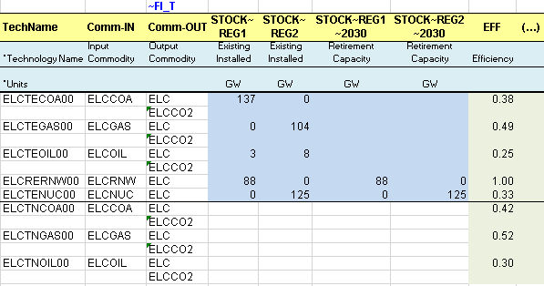
Figure 103. Regionalization of process attributes using additional columns
3.5.3.1. Scen_Trade_Links
The ~ TradeLinks tables are used to declare the traded commodities and their links between regions (Figure 104): either bilateral links between regions (e.g. ELC trade between REG 1 (importer/exporter) and REG2 (importer/exporter) or unilateral links between regions (e.g. GAS trade between REG 1 (importer) and REG2 (exporter). For each link declared (1=active links), VEDA2.0 will automatically create an IRE (inter-regional trade) process to which attributes may then be associated (e.g., bounds, investment costs, etc.). The naming convention for IRE processes is:
Bilateral trade: TB_<fuel name>_<exporter region>_<importer region>_<01> (e.g. TB_ELC_REG1_REG2_01)
Unilateral trade: TU_<fuel name>_<exporter region>_<importer region>_<01> (e.g. TU_GAS_REG2_REG1_01)
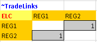
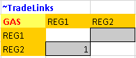
Figure 104. Examples of trade matrix for bilateral and unilateral links
3.5.3.2. Scen_Trade_Param
In this file, a transformation table ~TFM_INS is used to insert new attributes for trade processes (Figure 105), for example: an investment cost (INVCOST) for all unilateral trade processes (TU_*). Trade processes are created automatically after the user declares unilateral or bilateral links between regions in the _Trade_Links file.

Figure 105. Declaration of attributes for IRE processes
3.5.4. Scenario files
Two more scenario files are created to insert new information in the RES that can be retained or not in the configuration of the model at the time of solving the model. Of the previous scenario files, only the Scen_Peak_RSV file is retained for further analysis.
3.5.4.1. Scen_ELC_CO2_Bound
This file is used to introduce a bound (limit) on the CO2 emissions from the power sector in REG1. A transformation table ~TFM_INS is used (Figure 106) to declare an upper bound on annual emissions (Attribute = COM_BNDNET; LimType = UP), on the CO2 emissions from the electricity sector only (ELCCO2) in REG1. In this example the upper bound is calculated as a percentage reduction target from the power sector CO2 emissions in a reference scenario for 2010 (10% = 993,548 kt) and 2020 (20% = 1,017,340 kt). It is necessary to run the step model without any limit on emissions first to get the reference emission trajectory (run DemoS_005) and to calculate the bounds as a reduction target from the reference emissions. An interpolation rule is used with the “0” flag in the Year column and the interpolation/extrapolation option in the region column where the bounds are declared. The code 5 means full interpolation and forward extrapolation.
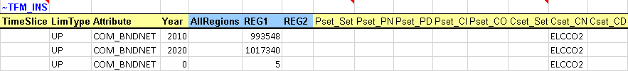
Figure 106. Declaration of emission bounds for the power sector
3.5.4.2. Scen_UCCO2_BND – user constraint
This file shows another way used to introduce bounds (limits) on the CO2 emissions from both the power and the transportation sectors in each region (REG1 and REG2). The idea is to build a user constraint (Figure 107) that specifies the maximum amount of emissions in a specific year for the sum of TRACO2 and ELCCO2 emission commodities.
These upper bounds (or limits) are again calculated as a percentage reduction target from the CO2 emissions (sum in kt) of the power and the transportation sector in a reference scenario for 2010 (10%) and 2020 (20%). It is necessary to run the step model without any limit on emissions first to get the reference emission trajectory (run DemoS_005) and to calculate the bounds as a reduction target from the reference emissions.
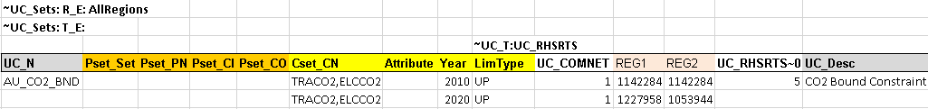
Figure 107. Declaration of emission bounds using a user constraint
The UC scenario template is set up as described in Section 2.4.7. The sets declarations above the table indicate:
~UC_Sets: R_E: AllRegions: The constraints are to be applied to all regions in the model, individually (E=each). That is, the bounds imposed for REG1 and REG2 are separate, and there is no emissions trading between regions.
~UC_Sets: T_E: The constraints are imposed to each time period individually. There is no banking or borrowing between periods.
The table level declaration following the table tag (~UC_T:UC_RHSRTS) indicates that any column without an index will be interpreted as the right hand side of the constraint, in this case, the indicated bounds in REG1 and REG2 in the given years. This right hand side bounds 1 times the net production (UC_COMNET) of the sum of TRACO2 and ELCCO2. The interpolation/extrapolation option 5 indicates full interpolation and forward extrapolation.
3.5.5. Results
Three cases are solved with this step model, with a different selection of scenario files: the DemoS_005 case is solved without any limit on CO2 emissions and using only the three main components (BASE, TRADE_PARAM, SysSettings), while the DemoS_005a case is solved adding one scenario file (ELC_CO2_BOUND) to put a limit on CO2 emissions from the REG1 power sector, and the DemoS_005b case is solved adding the other scenario file (UC_CO2_BND) to put a limit on both the power and the transportation sectors in both regions.
A first sample of results shows the different configuration of the energy supply systems in the two regions (Figure 108). As mentioned earlier, the REG1 becomes the main provider of solid fuels, renewable energies and some crude oil (from both domestic production and imports). REG1 is also getting electricity from REG2. REG2 becomes the main provider of natural gas, nuclear energy and some crude oil (from both domestic production and imports).
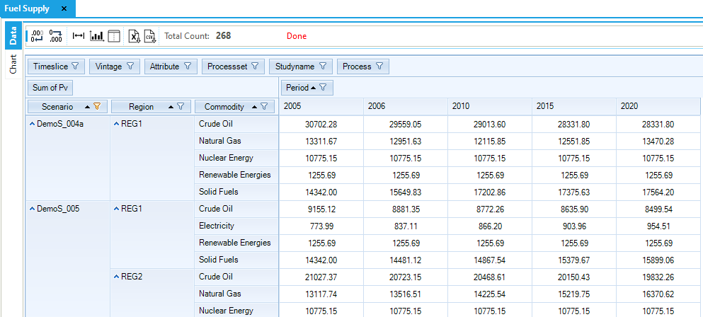
Figure 108. Fuel Supply (by Region) in DemoS_005
A second sample of results shows the evolution of the emissions in the different sectors of the two regions (Figure 109):
Emissions from the power and the transportation sectors as projected in the DemoS_005 case were used to compute the emissions limits in the other two cases.
A limit on the CO2 from the power sector in REG1 (DemoS_005a) leads to a lower electricity production from solid fuels, and an emission increase in REG2, which produces more electricity from natural gas to supply REG1 (Figure 110).
With a limit on the CO2 from both the power and the transportation sector in REG1 and in REG2 (DemoS_005b), all the emission reductions are coming from the power sector in both regions. Emissions from the transportation sector are not affected compared with the reference case (DemoS_005) meaning that the power sector of both regions could provide enough reduction options at a lower cost to meet the target. Because there is no trading in emissions between regions, REG2 must cut back on its electricity generation from natural gas, and it begins importing natural gas-fired electricity from REG1, which in turn imports natural gas from REG2 (Figure 110).
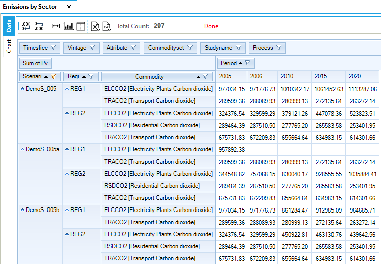
Figure 109. Emissions by Sector (and Region) in DemoS_005
Finally, the marginal price of CO2 (i.e. the price to pay in euros to reduce the last ton of CO2 to meet the reduction targets) in both scenarios with limits on emissions is particularly relevant and represents the level of tax that would be necessary to achieve the reduction targets that are prescribed in the scenario files (Figure 111).
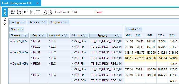
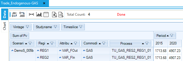
Figure 110. Endogenous Trades in DemoS_005
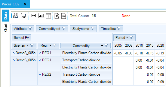
Figure 111. Emissions Price by Sector and Region in DemoS_005
Objective-Function = 3,204,949 M euros (see the _SysCost table) with 1,225,688 M euros for REG1 and 1,979,261 M euros for REG2. This cost is less than 0.1% higher with the emission limits for the power sector (3,206,161 M euros) and 1.4% higher with the emission limits for the power and the transportation sectors (3,250,281 M euros). More details about the impacts of the emission limits on the different cost components of the system in each region are shown below (Figure 112).
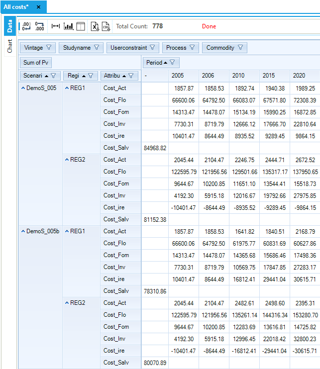
Figure 112. Costs by Sector and Region in DemoS_005
3.6. DemoS_006 - Multi-region with Separate Regional Templates
Description. At the sixth step, the configuration of the multi-regional model developed previously shifts from a single set of B-Y Templates for all regions to a separate sets of B-Y Templates for each region. This approach is relevant when the model regions are under the control of more than one individual.
Objective. The objective is again to create the multi-regional model framework typical to larger or more complex models, with the trade matrix and limits on emissions of all regions, but additionally to introduce the concept of technology repositories (i.e., SubRES) that include a number of new processes (in competition) that are available in the database to replace the existing ones at the end of their lifetime or to meet an increasing demand.
The motivation behind these repositories is mainly to avoid repeating the new process specifications for each region; all attributes specifications apply to all regions unless a transformation file is used to regionalize some values when necessary.
Simultaneously, the role of the vintage feature is illustrated to handle processes for which characteristics change over time (other than investment cost) when new capacity is built. As in step 5, the scenario variants illustrate the impact of a cap on CO2 emissions from the electricity sector only and of a cross-region user constraint on the total CO2 emissions from the transport and electricity sectors.
Attributes Introduced |
Files Updated |
|---|---|
N.A. |
SysSettings |
Files Created |
|
SubRES_NewTechs |
|
VT_REG1_PRI_v06 |
|
VT_REG2_PRI_v06 |
|
Files Replaced |
|
VT_REG1_PRI_v05 |
Files. The sixth step model is built 1) by modifying the SysSettings file to add one B-Y Template, 2) by replacing the B-Y Template (VT_REG_PRI_V05) by two B-Y Template (VT_REG1_PRI_v06, VT_REG2_PRI_v06) to disaggregate the energy balance between two regions in two separate files, and 3) by creating a SubRES file to add new processes to the model (Figure 113). Note that for the rest of this manual the region templates will be stated as REG1/2, rather than listing each separately.
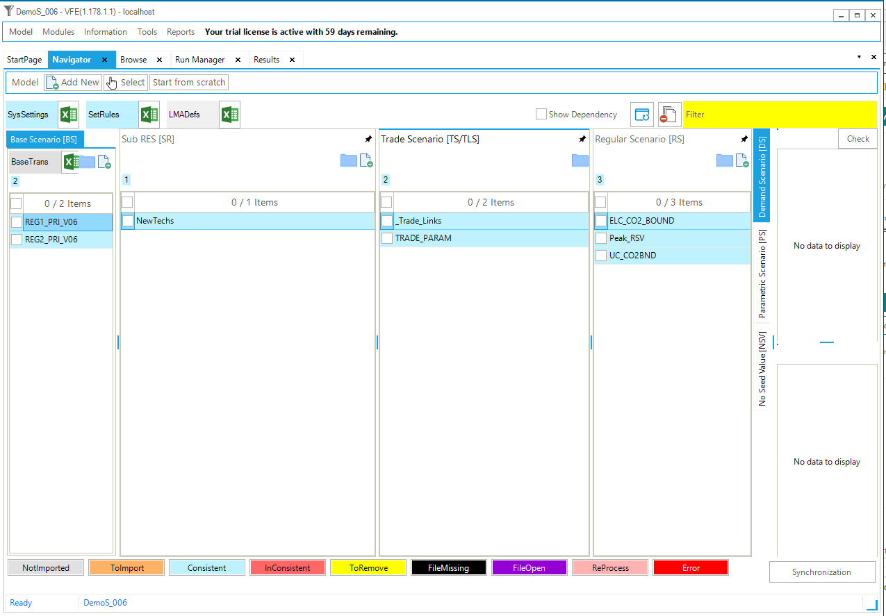
Figure 113. Templates Included in DemoS_006
3.6.1. SysSettings file
3.6.1.1. Region-Time Slices
The ~BookRegions_Map table is used to create one additional workbook: one for each region REG1 and REG2 (Figure 114).
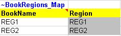
Figure 114. New workbook name definitions in the SysSettings file
3.6.2. B-Y Templates
The structure of the two B-Y Templates (VT_REG1_PRI_v06 and VT_REG2_PRI_v06) is identical to the structure of the B-Y Template of the fourth step model and uses the same energy balances defined in the fifth step model for REG1 and REG2 respectively. There is no change to report, except that new power plants are moved from the B-Y Template to the new process repository.
3.6.3. SubRES_NewTechs
Two files are created to add new processes in the model, the SubRES and SubRES_Trans files. The SubRES file is a repository of new processes available for all regions. In the SubRES, by default, all attribute specifications apply to all regions. This approach is convenient for models with multiple regions because a single set of declarations can be made for all regions. The SubRES file includes one sheet for each sector: PRI_ELC, PRI_RSD, PRI_TRA, PRI_FuelSec. (Due to the way SubRES are processed in VEDA2.0, it is required that the name of each sheet start with a valid name of one of the model sectors, as defined in the names of the B-Y templates. In this case, PRI is the only such model sector, and so all sheets in the SubRES template begin with PRI_.)
With this approach, the B-Y Templates now include only processes with existing capacity in the base year 2005, and all new processes are defined in the SubRES. Duplicate definition should be avoided. The new power plants are now declared in this file without any regional specification (Figure 115). Other new processes are created in the other sheets following the same rules: new processes do not have an existing installed capacity, but they are characterized with an investment cost (INVCOST) as well as the year where they become available (START).
The role of the vintage feature is illustrated to handle processes for which characteristics other than investment cost change over time when new capacity is built., In this example, the new gas-fired power plant (ELCTNGAS00) has its efficiency and emission coefficient evolving between 2006 and 2020. The process ELCTNGAS00 is vintaged (Vintage=Yes) in the ~FI_Process table (Figure 116).
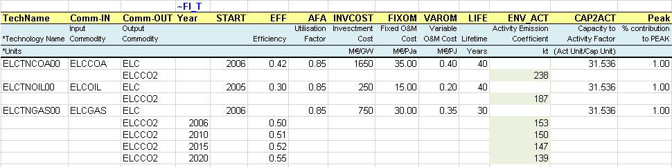
Figure 115. Example of new processes in the SubRES file
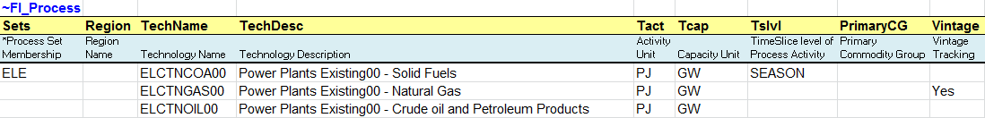
Figure 116. Example of a new process with vintage tracking in the SubRES file
3.6.3.1. SubRES_NewTechs_Trans
For each SubRES_<user-name> file, there is an associated SubRES_<user-name>_Trans file. The transformation files contain the mapping and transformation operations that control the inheritance (or not) of new processes into the various regions of the model, as well as to change any process characteristics, such as investment costs, by region. In this example, the file is empty, so all new processes in the SubRES are available in both regions with identical characteristics.
3.6.4. Results
The results are very similar to those obtained with the previous step model since most of the changes occurred in the way the information is structured in different files rather than in the energy system itself. However, the impact of the vintage feature for the new gas-fired power plants is illustrated (Figure 117).
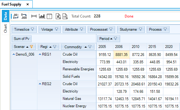
Figure 117. Fuel Supply by Region in DemoS_005
Objective-Function = 3,205,281 M euros (see the _SysCost table) with 1,293,017 M euros for REG1 and 1,912,264 M euros for REG2. These costs are similar to those computed with the previous step model DemoS_005.
3.7. DemoS_007 – Making DemoS More Robust
Description. The seventh step model is enhanced to capture more components of the energy balance, leading to a more comprehensive representation of the RES with more complex processes.
Objectives. The objective is to show how to model a more comprehensive RES covering more details of the energy balance with more complex processes along its two dimensions: number of commodities and the number of transformation steps in the whole supply-demand chain. In this step refined petroleum products are broken out into different commodities (e.g., gasoline, diesel, heavy fuel, etc.) to better describe the transport sector, where different types of vehicles are introduced. This enhancement of the RES requires the modelling of additional and more complex processes (e.g., refineries and dual demand cars) and the need to introduce the primary commodity group (PCG) concept.
Several more techniques are also introduced in this step:
We present an easier way to account for combustion-based emissions, by directly linking emission coefficients with each unit of fuel burnt.
We illustrate how to build end-use demand projections starting from base year values and different growth rates. This is done using the fill table feature to grab base year information from the initial files (e.g. B-Y Templates).
We show how to build a user constraint that specific the minimum (or maximum) annual growth rate for a set of processes using the CAP, GROWTH attribute.
Finally, we demonstrate how to use the elastic demand feature of TIMES, including how to generate the file containing the demand prices for base scenarios and how to use these prices for the constrained scenarios.
Attributes Introduced |
Files Updated |
|---|---|
Share |
SysSettings |
ACTFLO |
VT_REG1/2_PRI_v07 |
COM_VOC |
SubRES_NewTechs |
COM_STEP |
Files Created |
COM_ELAST |
Scen_DemProj_DTCAR |
UC_CAP |
Scen_Refinery |
Scen_ElasticDem |
|
Scen_TRA_CO2_BOUND |
|
Scen_UC Growth |
Files. The seventh step model is built:
by modifying the SysSettings file to add interpolation rules;
by modifying the two B-Y Template (VT_REG1_PRI_v07, VT_REG2_PRI_v07) and the SubRES file (SubRES_NewTechs) to add more commodities, more complex processes, and emission coefficients, and to introduce the PCG concept;
by creating a scenario file to project demand from base year values;
by creating a scenario file to update refinery attributes;
by creating a scenario file to include price-elasticities for demands;
by creating a scenario file with a limit on emissions from thetransportation sector;
by creating a scenario file with a user constraint on growth rates of new cars (Figure 118).
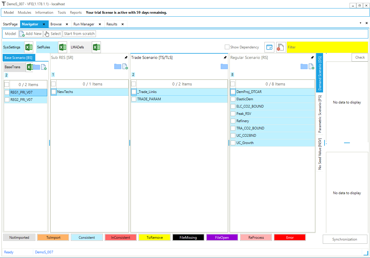
Figure 118. Templates Included in DemoS_007
3.7.1. SysSettings file
3.7.1.1. Interpol_Extrapol_Defaults
More interpolation/extrapolation rules are added to the transformation table (Figure 119). The same interpolation/extrapolation rule (number 5) is also used for the maximum input shares (Share-I) and the maximum output shares (Share-O) of all processes at once. These new attributes are defined in the next section.
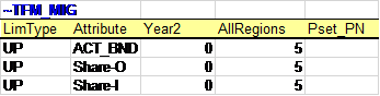
Figure 119. Updated Interpolation/Extrapolation Rules
3.7.2. B-Y Templates
3.7.2.1. EnergyBalance
At this step, the energy balance is disaggregated and includes a larger number of commodities. The crude oil category is disaggregated to track all refined products independently (Figure 120) to better describe the transport sector where different types of cars are introduced. A larger portion of the energy balance is covered in terms of the number of commodities and also of the number of transformation steps in the whole supply-demand chain, with the addition of the refining step.
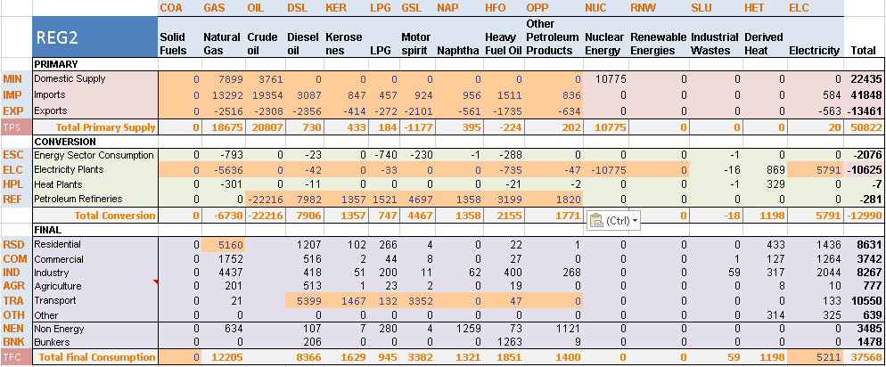
Figure 120. Disaggregated Initial Energy Balance (2005) for REG2 in DemoS_007
3.7.2.2. Con_REF – primary commodity group definition
A flexible refinery (REFEOIL00) is introduced in this sheet (Figure 121) to convert crude oil (OIL) into refined products (DSL, KER, LPG, GSL, etc.) that will be used in the transportation sector.
The existing refinery is characterized with an efficiency (EFF) and an annual activity bound (ACT_BND) equivalent to the sum of the refined products produced at base year 2005 as given in the energy balance. In this example the efficiency is represented by the ratio of the crude oil in input to the refinery on the sum of the petroleum products in output. For this reason we get an efficiency greater than 1. This behaviour depends on the definition of the commodity group of a technology (see below for more details).
This more complex process with multiple outputs commodities is also characterized with a new attribute: the maximum share for each commodity output in the total production (Share-O~UP). In this example, the maximum shares for all outputs sum to 100%, meaning that they are equivalent to fixed shares. It would be possible to have a sum of maximum shares greater than 100%, leaving some flexibility to the model to optimize the output mix.
The same approach is used to declare the new commodities and processes in their definition tables, where the refinery is declared as a PRE process, and the concept of Primary Commodity Group (PCG) is introduced (Figure 122). The activity of a standard process is equal to the sum of the commodity flow(s) on either the input side or the output side of a process, as defined by the PCG. The activity of a process is limited by the available capacity, so that the activity variable establishes a link between the installed capacity of a process and the maximum possible commodity flows entering or leaving the process during a year or a subdivision of a year.
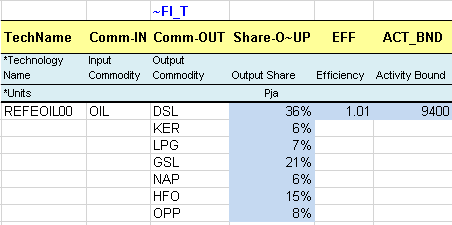
Figure 121. Refinery
In a simple process, one consuming a single commodity and producing a single commodity, the modeler simply chooses one of these two flows to define the activity, and thereby the process normalization (input or output). In complex processes, with several commodities (perhaps of different types) as inputs and/or outputs, the definition of the activity variable requires designation of the PCG to serve as the activity-defining group. The PCG is defined as a subset of the commodities of the same nature entering or leaving a process. For instance, the PCG may be the group of energy carriers, or the group of materials of a given type, on either the input or output side of the process. More about PCGs and their use can be found in Section 2.2.1 of Part II of the TIMES documentation.
VEDA2.0 establishes default PCGs for any process involving multiple inputs and/or outputs, based upon the assumption first that all processes are output normalized and then according to the commodities’ nature. In case of different commodity types on the output (or input) side, the default PCG is based on the following order:
DEM – demands;
MAT – materials;
NRG – energy;
ENV – emissions, and
FIN – financial.
However, in some cases it is desirable/necessary to override these defaults, for instance to normalize a process with energy commodities inputs (NRGI) as for the refinery in this example. Indeed, the activity of a refinery is usually characterized based on the barrels of crude oil consumed.
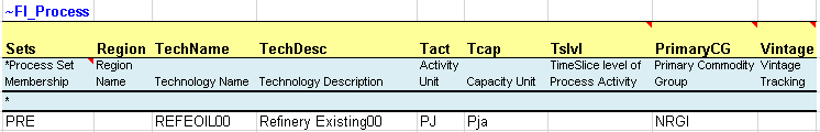
Figure 122. Set PCG for the Refinery
3.7.2.3. Pri_PP
Import and export options for all refined petroleum products were added in this sheet; they are characterized with the COST and ACT_BND attributes as for any other primary fuels (solid fuels, natural gas, crude oil) (Figure 123). Note that by convention, the export prices are generally be slightly less than import prices, to avoid the model importing just to export.
3.7.2.4. Sector_Fuels
Additional sector fuel processes (FTE-*) are defined and characterized in this sheet (Figure 124), namely to produce the transportation sector fuels from primary refined products (e.g. GSL to TRAGSL). It is not always relevant to keep track of all primary fuels in a sector; multiple primary fuels can be aggregated into a single sector fuel in this case. In this example, several refined products are aggregated into a single electricity sector fuel (via FTE-ELCOIL). When more than one primary fuel are used to create one sector fuel, the shares of input fuels (Share-I~UP) need to be provided. As with Share-O, the maximum input shares may sum to greater than 100%, if desired, to provide some process flexibility.
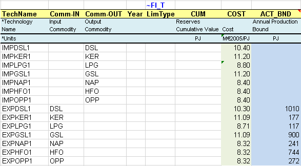
Figure 123. Imports and Exports of Refined Petroleum Products
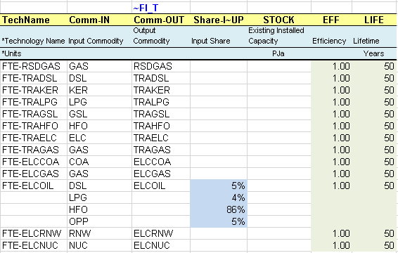
Figure 124. Additional Sector Fuel Processes with Multiple Input Commodities
3.7.2.5. DemTechs_TRA
The single demand process consuming an energy commodity (TRAOIL) and producing directly the transport demand commodity (DTD1) is replaced with more sophisticated processes representing cars and characterized with non-energy units (Figure 125). The declaration of these processes is shown below (Figure 126): their activity units are in billions passengers-kilometres (BpK) rather than PJ, and their capacity units are in thousands of units (000_units) rather than PJa.
The existing processes are characterized with their existing installed capacity (STOCK) in thousands of car units (000_units) as indicated above. The stock values correspond to the amount of fuel consumption (e.g. TRADSL) required to produce the transportation demand (DTCAR) as given by the energy balance and taking into account the efficiency (EFF), the annual availability factor (AFA) and the conversion between capacity unit and activity unit (CAP2ACT).
The efficiency (EFF) is specified in terms of billions of vehicle-kilometres per petajoule (BVkm/PJ), and can be interpreted as the number of kilometres a vehicle can travel with 1 PJ of energy.
The annual availability factor (AFA) represents the average thousand kilometres (‘000 km) a car is traveling each year.
A new attribute is introduced to capture the relation between the process activity and the commodity flow (ACTFLO), the commodity being the output demand, in terms of passengers per car unit (Passenger/Car). This TIMES parameter requires an additional index that is the specification of the commodity group: DEMO (demand out) in this example.
The life time (LIFE) is specified in number of years as for the other processes.
The conversion factor between capacity unit and activity unit (CAP2ACT) is not equal to 1 because the units are different: the activity is in billion vehicle-kilometres, the stock is in thousands of units (000_units or vehicles) and the utilization factor (AFA) is in thousand kilometres per vehicle. The CAP2ACT is translating mvkm into bvkm.
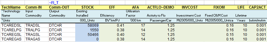
Figure 125. More Complex Transportation Processes
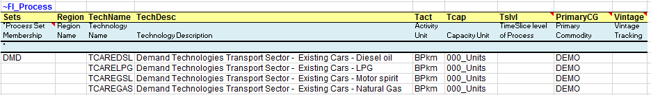
Figure 126. Declaration of More Processes in the Transportation Sector
3.7.2.6. Demands
The demand for transportation by cars is updated and declared in the right units and correspond to the sum of billion passengers-kilometres (Bpass*km) for all types of cars (Figure 127):
Demand (Bpass*km) = STOCK (000_units) * AFA (000_vehiclekm/unit) * ACTFLO~DEMO (Passengers/vehicle)* CAP2ACT(0.001bvkm/mvkm)
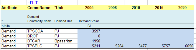
Figure 127. Demand for Transportation by Car (physical units)
3.7.2.7. Emi
A new sheet is added to introduce a comprehensive and convenient approach to account for combustion emissions by sector. Indeed, the easiest way to account for combustion emissions is to directly associate the fuel-based emission coefficients with fuel consumption throughout the whole energy system.
A new ~COMEMI table is added (Figure 128) to define fuel-based emission coefficients instead of defining emission coefficients for each process in all ~FI_T tables. The special tag ~COMEMI is used to link emissions to commodity consumption through special processing in the VEDA2.0 SYNC process. (The VEDA-TIMES parameters VDA-EMCB and FLO-EMIS provide alternative ways to declare consumption-linked emissions. See Part II of the TIMES documentation for more on the use of these parameters.)
In this example, emissions of TRACO2 are associated with six fuels (LPG, gasoline, kerosene, diesel, heavy fuel oil, natural gas,) for which a coefficient (kt/PJ) is provided. These coefficients are applied to all the fuel consumption by all the individual processes in the transportation sector.
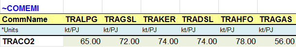
Figure 128. Combustion Emissions from the Transportation Sector
3.7.3. SubRES_NewTechs
3.7.3.1. PRI_TRA
This sheet is updated to model the new cars using the same approach as described above for the existing cars.
3.7.4. Scenario files
Several scenario files are created at this seventh step.
3.7.4.1. Scen_DemProj_DTCAR
This scenario file is created to project transport demand using a fill table to grab base year values from B-Y templates (Figure 129). The ~TFM_FILL table (see section 2.4.6 for more information) is a feature allowing a template to collect information from other templates. In this example, the table is collecting the base year values (YEAR=2005) from the B-Y templates (Scenario = BASE) for the transportation demand (Attribute=Demand) by cars (commodity = DTCAR). VEDA2.0 fills in the REG1 and REG2 values in the blue highlighted cells each time the template is SYNCed.

Figure 129. Grab Base Year Demand Values from B-Y Templates - Transportation
The DTCAR demand is then projected to 2020 in the ~TFM_INS table using the base year values and some multipliers (2% for REG1 and 3% for REG2) defined by the user (Figure 130).
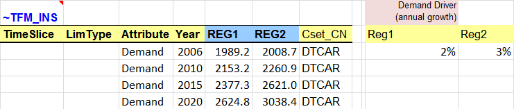
Figure 130. Using Base Year Values to Project End-use Demands - Transportation
3.7.4.2. Scen_Refinery
This scenario file is created to update refinery attributes, again using a fill table to grab information from B-Y templates (Figure 131). In this example, the table is collecting the base year values (YEAR=2005) from the B-Y templates (Scenario = BASE) for the activity production bound (Attribute=ACT_BND) of the refinery (process = REFEOIL00).
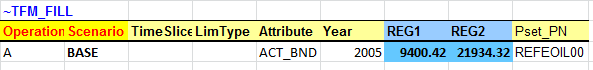
Figure 131. Grab Base Year Activity Level from B-Y Templates - Refinery
The activity production is then projected to 2020 in the ~TFM_INS table using the base year values and some relaxation factors (25% for REG1 and 30% for REG2) defined by the user (Figure 132). In addition, the maximum (UP) shares of the refinery outputs (Attribute=SHARE-O) are all updated to 50%, creating flexibility for the model to optimize the mix of refined products (DSL, KER, LPG, etc.).
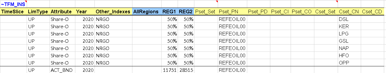
Figure 132. Using Base Year Values to Update Refinery Attributes
3.7.4.3. Scen_TRA_CO2_BOUND
This file is used to introduce bounds (limits) on the CO2 emissions from the transportation sector in REG1 and REG2. A transformation table ~TFM_INS is used (Figure 133) to declare upper bounds on annual emissions (Attribute = COM_BNDNET; LimType = UP), on the CO2 emissions from the transportation sector only (TRACO2) in REG1 and REG2. These upper bounds are calculated as percentage reduction targets from the transportation sector CO2 emissions in a reference scenario for 2010 (10%) and 2020 (20%). It is necessary to run the step model without any limit on emissions first to get the reference emission trajectory (run DemoS_007) and then calculate the bounds as a reduction targets from the reference emissions. An interpolation rule is used with the “0” flag in the Year column and the interpolation/extrapolation option in the region column where the bounds are declared; the code 5 means full interpolation and forward extrapolation.
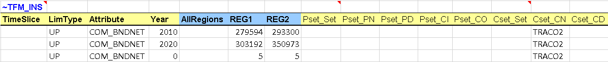
Figure 133. Set Emission Bounds for Transportation Sector
3.7.4.4. Scen_UC Growth
This file shows another type of user constraint that specifies the maximum (or minimum) annual growth rate for a set of processes using the CAP, GROWTH attribute (Figure 134). (See Section 2.4.7 for more on user constraints.)
This user constraint imposes a maximum capacity (defined by UC_CAP) growth rate (CAP,GROWTH) of 1% per year (value in the column UC_CAP) for cars consuming TRADSL (these cars are identified using the two columns PSET_CO and PSET_CI). This constraint also provides a seed value of 1 (column UC_RHSRTS) to enable the capacity growth to start in case the existing capacity of diesel cars is zero.
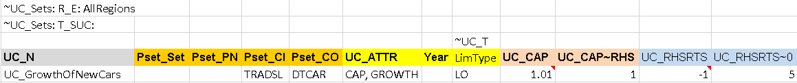
Figure 134. Specifying Growth Rates with a User Constraint
3.7.4.5. Scen_ElasticDem
This file is used to introduce price-elasticities for end-use demands (Figure 135), so that demands can react to changes in their prices under a constrained energy system (e.g., under limits or tax on emissions, etc.). (See Section 4.2 of Part I of the TIMES documentation for more on the elastic demand formulation.)
In this example, price-elasticities are declared for the transportation demand by cars (DTCAR). Three attributes need to be declared:
COM_ELAST: Elasticity of demand indicating how much the demand rises/falls in response to a unit change in the marginal cost of meeting a demand that is elastic.
COM_VOC: Maximum possible variation of demand in both directions when using the elastic demand formulation (15% in this example).
COM_STEP: Number of steps for the linear approximation of the demand curve (10 steps in this example).
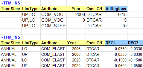
Figure 135. Declare Price-elasticities for End-use Demands
In order to activate the elastic demand feature, there are few steps to follow:
Generate a file with demand prices from a reference case, i.e. without any constraint or tax on emissions: in the Parameter Group make sure the option “Write B Price for Elast Dem” is selected (Figure 136). This option is already selected in the DemoS_007.
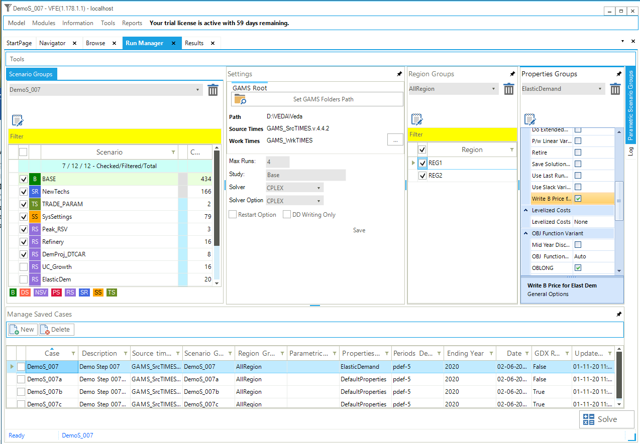
Figure 136. Write Base Prices for Elastic Demands
Solve a constrained case with price-elasticity by selecting the constrained scenarios you want to include in the model run (emission limits or taxes) as well as the elastic demand scenario. In the RunManager Case DemoS_007a is an emission constrained case run without elastic demands, while Case DemoS_007b B prices and emissions constraint scenario, see Figure 137.
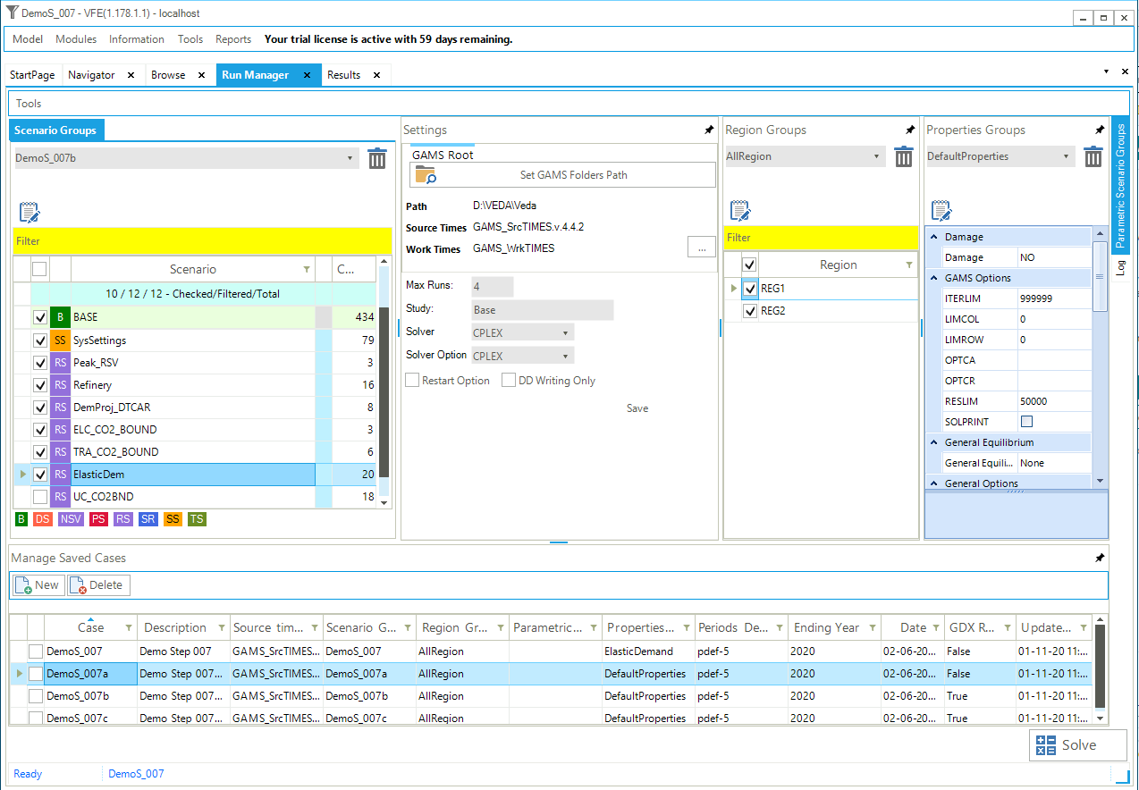
Figure 137. Include the B Elastic Demand and Emission Constraint
3.7.5. Results
The effect of price elasticities on the new projected demand for car transportation in thousand passengers-kilometres (kpass*km) to the 2020 horizon is visible (Figure 138) in the scenarios where it was activated (DemoS_007b and DemoS_007c). Demands are decreasing by about 9% in both regions, less than the maximum decrease of 15%, meaning than more cost-effective emission reduction options exist elsewhere in the system beyond that level.
The impacts of the emissions constraints and the growth rate constraint on the optimal process mix selected to meet the car transportation demand (kpass*km) is shown (Figure 139) for both regions together:
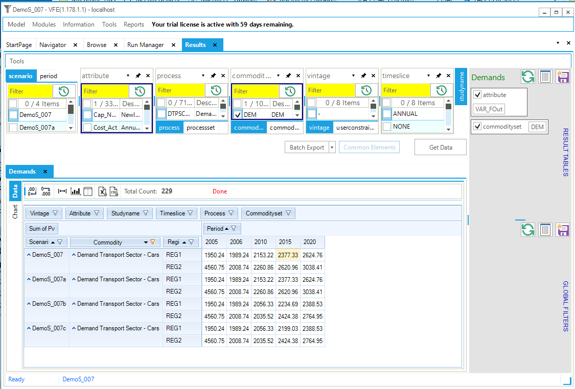
Figure 138. Results - Effect of Price Elasticities on Car Transportation Demand in DemoS_007
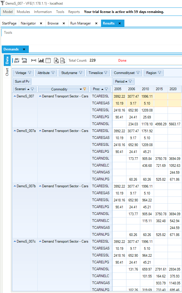
Figure 139. Results – Car Transport Vehicle Type Mix in DemoS_007
In the reference case (DemoS_007), new diesel cars satisfy the entire demand for car transportation from 2015 and beyond. The output mix of the refinery is shown below (Figure 140).
The limits on the transportation sector emissions (DemoS_007a) lead to a switch toward less polluting options such as electric, natural gas and LPG cars.
The activation of elastic demand (DemoS_007b) leads to a reduction in the use of the most expensive option to meet demand – electric cars.
The addition of a growth rate constraint on diesel cars (DemoS_007c) leads to a switch toward natural gas cars.
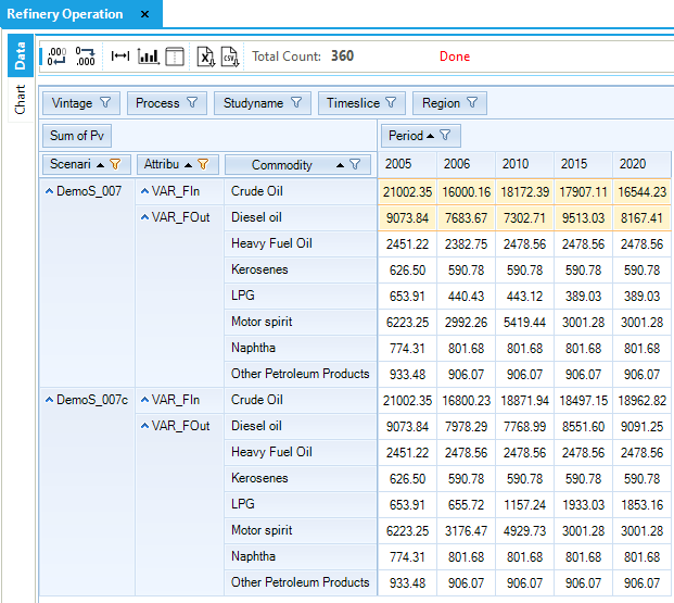
Figure 140. Flexible Refinery Operation in DemoS_007
Objective-Function = 5,484,966 M euros (see the _SysCost table) with 2,859,389 M euros for REG1 and 2,625,577 M euros for REG2. These costs are higher than those computed with the previous step model DemoS_006 because of the many components added to the RES. The total cost is 12% higher when emissions limits are imposed on the transportation sector (6,145,863 M euros), but only 7% higher with the activation of elastic demand as the model has more flexibility to reach the emissions targets (5,891,267 M euros). The addition of the growth rate constraint on diesel cars brings the system cost increase back up to 10% (6,025,956 M euros).
3.8. DemoS_008 - Split Base-Year (B-Y) templates by sector: demands by sector
Description. At the eighth step, the level of detail in the representation of the RES is expanded further, the base-year information is disaggregated into different B-Y Templates for each sector, and demands are projected through 2050. Each of these B-Y Templates utilizes only the relevant portion of the energy balance for its region and is linked to an additional single file containing the complete regional energy balances. This approach is convenient when different individuals work in parallel on different sectors. In addition, it encourages grouping of related commodities and processes, and as the size of a model grows it improves (and speeds up) the process of managing the model.
Objective. The objective is to give more examples on how to further expand the detail of the representation of the RES, in terms of the number of end-use demand segments and end-use devices as well as commodities. On the demand side, the idea is to cover the energy consumption by end-use in all sectors rather than by type of energy: agriculture (one end-use demand), commercial (three end-use demands), residential (three end-use demands), industrial (one end-use demands), and transport (two end-use demands). On the supply side, the idea is to break the renewables into more detail for wind, solar, hydro and biomass power. This enhancement of the RES requires the modelling of additional processes as well as the addition of emission coefficients for all sectors.
Another objective is to show how to impose a limit on power generation capacity: nuclear, for example. The scenario variants with nuclear maximum capacity, with different types of limits on emissions, and with and without the elastic demand feature, illustrate the impacts on the respective contribution of each sector to the target as well as on the electricity generation mix.
Attributes Introduced |
Files Updated |
|---|---|
N.A. |
SysSettings |
Scen_TRA_CO2_Bound |
|
Scen_ELC_CO2_Bound |
|
Scen_UC_CO2BND |
|
SubRES_NewTechs |
|
Files Created |
|
VT_REG1/2_PRI_v08 |
|
VT_REG1/2_ELC_v08 |
|
VT_REG1/2_RCA_v08 |
|
VT_REG1/2_TRA_v08 |
|
VT_REG1/2_IND_v08 |
|
Scen_UC_NUC_MaxCAP |
|
Files Replaced |
|
VT_REG1/2_PRI_v07 |
Files. The eighth step model is built:
by modifying the SysSettings file to add more time periods;
by replacing the two B-Y Templates (VT_REG1_PRI_v07, VT_REG2_PRI_v07) by five B-Y Templates – one for each sector – in each region (VT_REG1_*_v08, VT_REG2_*_v08), and to add more energy commodities, energy processes, and emissions;
by completing the SubRES file;
by updating scenario files with limits on emissions;
by creating a scenario file with a user constraint on the maximum nuclear power capacity (Figure 141).
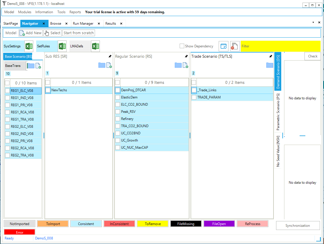
Figure 141. Templates Included in DemoS_008
3.8.1. SysSettings file
3.8.1.1. TimePeriods
The ~TimePeriods table is used to extend the time horizon of the model by adding six active periods of five years (Figure 142). These specifications are saved under a new time period definition (Pdef-11). The time horizon is extended to 2050 with the milestones years being 2005, 2006, 2010, 2015, 2020, 2025, 2030, 2035, 2040, 2045 and 2050. This can be seen in VEDA2.0, Advanced Functions menu, MileStone Years tab.
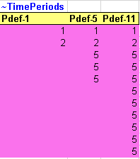
Figure 142. New Time Periods Definition in SysSettings
3.8.1.2. Defaults
The ~DefUnits table is used to specify the different default activity, capacity and commodity units for each sector in the model (Figure 143).
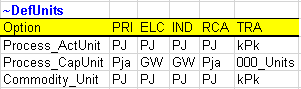
Figure 143. Default Declarations in SysSettings
3.8.2. B-Y Template VT_REG*_PRI_V08
3.8.2.1. EnergyBalance
The energy balance is disaggregated further and includes a larger number of commodities. The renewable category is disaggregated to track several sources independently: biomass as well as hydro, wind, and solar energy (Figure 144). Moreover, the energy balances of both regions are now moved into a separate file (called EnergyBalance) and all B-Y Templates are linked to this file to grab the relevant sector data.
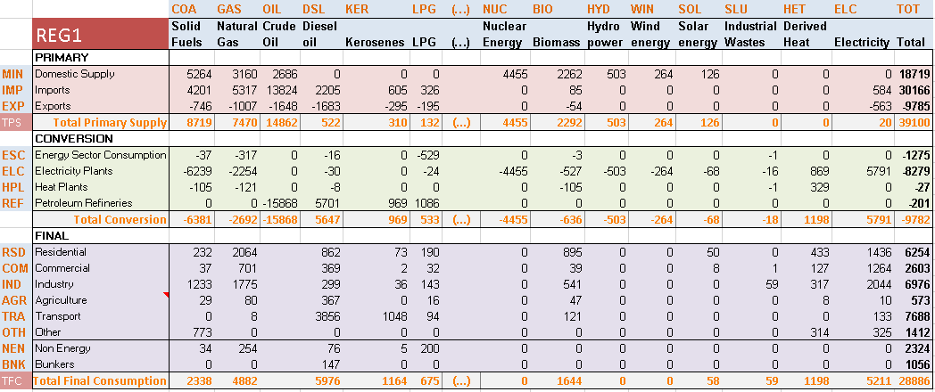
* For purposes of clarity the energy balance is not presented totally and some columns are missing (for refined products).
Figure 144. Disaggregated Initial Energy Balance (2005) for REG1 in DemoS_008
3.8.2.2. Pri_COA, Pri_GAS, Pri_OIL, Pri_PP, Con_REF
The structure of these sheets have not changed, but the data is updated following a different commodity split between REG1 and REG2 in the energy balance.
3.8.2.3. Pri_RNW and Pri_NUC
Mining processes for the uranium resources and the new renewable potentials are characterized with a cost (Figure 145).
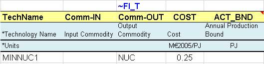
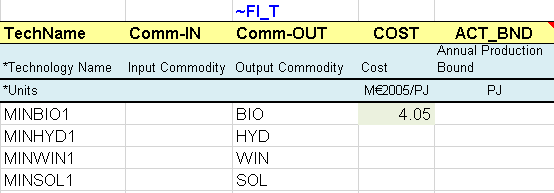
Figure 145. New Renewables Supply Options
3.8.2.4. Pri_ELC
This sheet is created to capture the imports and exports of electricity (Figure 146). In the default process table, the operational level of these processes are declared as DAYNITE in the Tslvl column. Note that the ELC commodity is not declared in the default commodity table as it is already declared in the ELC B-Y Templates. Commodities need to be declared only once and then are available for all files (not only B-Y Templates).
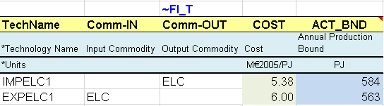
Figure 146. Electricity Imports and Exports Options
3.8.3. B-Y Template VT_REG*_ELC_V08
3.8.3.1. Con_ELC
New power plants are added for each type of renewable energy (Figure 147) using the same approach as before. Their contribution to peak varies depending on the resources: 50% for hydro, 30% for wind, and 20% for solar. However, there is no emission coefficient associated with process anymore (in ~FI_T tables). All combustion emissions are tracked in a uniform manner at the sector level in a ~COMEMI table.
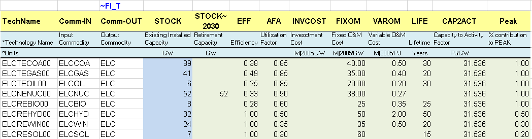
Figure 147. New Renewable Electric Generation Power Plants
3.8.3.2. Emi
A similar sheet is added in all sectors with a ~COMEMI table used to define fuel-based emission coefficients associated with fuel consumption in each sector (Figure 148).
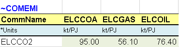
Figure 148. Combustion Emissions from the Electricity Sector
3.8.4. BY Template VT_REG*_IND_V08
3.8.4.1. DemTechs_IND
The energy consumed in the industrial sector is captured through a single generic process (Figure 149) consuming the mix of industrial fuels as given in the energy balance and producing one end-use demand (DIDM1). A relaxation factor is used for the maximum input shares in 2050 to give more flexibility to the model over time to optimize the fuel mix. However, the value of the relaxation factor should remain realistic since most fuel switches involve process switches as well.
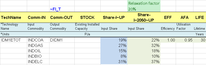
Figure 149. Flexible Multiple Input Process in the Industrial Sector
3.8.4.2. Emi
An emission commodity is created (Figure 150) and a ~COMEMI table is added in the Emi sheet to track all fuel-based emissions from the sector.
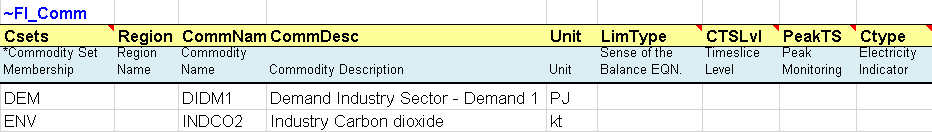
Figure 150. New Environmental Commodity for Industrial Emissions
3.8.5. BY Template VT_REG*_RCA_V08
This B-Y Template includes the information related to three sectors: agriculture, commercial and residential.
3.8.5.1. DemTechs_AGR
The energy consumed in the agriculture sector is captured through a single generic process (as for the industrial sector) consuming the mix of agriculture fuels as given in the energy balance and producing one end-use demand (DAOT). A relaxation factor is also used for the maximum input shares in 2050 to give more flexibility to the model over time to optimize the fuel mix. However, the value of the relaxation factor should remain realistic since most fuel switches involve process switches as well.
3.8.5.2. DemTechs_RSD and DemTechs_COM
The energy consumed in the commercial and the residential sectors is modelled through specific processes (Figure 151). Multiple processes are in competition to satisfy each end-use demand (e.g., RSHE* to satisfy the DRSH demand). The existing processes are characterized with their existing installed capacity (STOCK) corresponding in this case to the energy consumption required to produce these energy services as given by the energy balance and the additional fuel split assumptions. The calculation of the existing stocks also takes into account availability factors (AFA) and are converted into GW using a capacity to activity factor (PRC_CAPACT equivalent to CAP2ACT). They also have an efficiency (EFF) and a life time (LIFE).
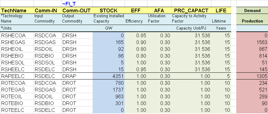
Figure 151. Existing Residential Sector Processes
3.8.5.3. Demands
The demand table includes all end-use demands for energy services from the three sectors (Figure 152). The values come from the process sheets where the values are already computed in the pink column (Figure 151): STOCK*AFA*PRC_CAPACT. This sheet also includes the fractional shares of each end-use demand by time slice (Figure 153). These shares are relevant to capture the annual variation in the electricity (ELC) consumption levels and prices, the only commodity tracked at the time slice level. In this example, the annual variations are significant for those end-use demands affected by seasonal changes (e.g. space heating).
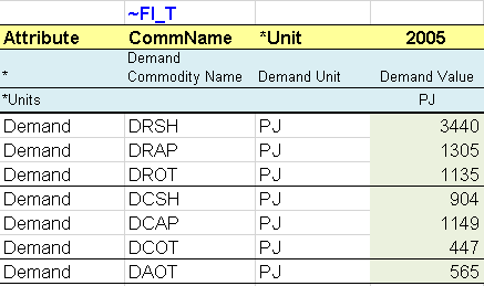
Figure 152. Demand for Energy Services in the RCA Sectors
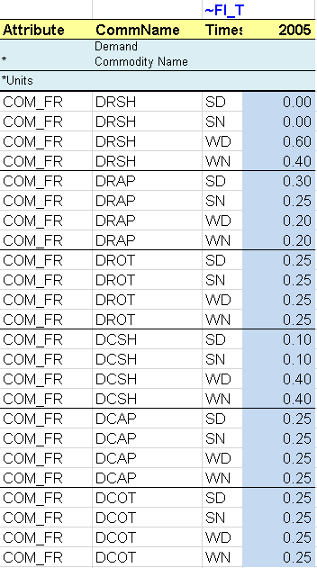
Figure 153. Fractional Shares for RCA Energy Service Demands
3.8.5.4. Emi
An emission commodity is created in all three sectors and three ~COMEMI tables are added in the Emi sheet to track all fuel-based emissions from each of the three sectors.
3.8.6. BY Template VT_REG*_TRA_V08
3.8.6.1. DemTechs_TRA
The energy consumed in the transportation sector is disaggregated into two end-use demands: transportation by cars and public transport. Consequently, more existing processes are included to satisfy the demand for the new public transport demand, and they are modelled using the same approach as for cars (Figure 154).
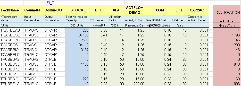
Figure 154. Existing Transportation Sector Vehicle Types
3.8.6.2. Demands
The demand table includes both end-use demands (in Bpass-km) and the fractional shares of each end-use demand by time slice.
3.8.6.3. Emi
An emission commodity is created and a ~COMEMI table is added in the Emi sheet to track all fuel-based emissions from the sector.
3.8.7. SubRES_NewTechs
The structure of this file has not changed; this is a repository of new processes available for all the regions. The file includes one sheet for each sector: ELC, PRI, IND, RCA, TRA. (The sheet’s names have changed and reflect each new sector’s name).
The new process repository is completed with more new processes similarly as for the existing processes in the B-Y Templates, namely more processes for renewable power generation, public transport, and more energy services in the residential and commercial sectors (Figure 155).
3.8.7.1. IEA-ETSAP_ETechDS
This sheet contains a reference to the technology briefs (E-TechDS – Energy Technology Data Source) coordinated by the ETSAP-IEA. They are classified into two main categories: energy supply technologies and energy demand technologies. They provide relevant data on the most important technical and economic attributes of numerous types of technologies.[3]
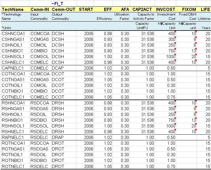
Figure 155. New Residential and Commercial Devices
3.8.8. Scenario files
3.8.8.1. Scen_UC_CO2BND
This user constraint is updated to introduce bounds (limits) on the CO2 emissions from all sectors in each region (REG1 and REG2). These upper bound are calculated as a percentage reduction target from the CO2 emissions (sum in kt) from all the sectors in a reference scenario for 2010 (10%) and 2020 (20%). It is necessary to run the step model without any limit on emissions first to get the reference emission trajectory (run DemoS_008) and to calculate the bounds as a reduction target from the reference emissions.
3.8.8.2. Scen_UC_NUC_MaxCAP
To build this scenario, a ~TFM_FILL table first collects information from the B-Y Templates for REG1 and REG2 (Figure 156): the installed capacity (STOCK) of the nuclear power plant (ELCNENUC00). These data are refreshed each time this file is synchronized (SYNC). Second, a user constraint is built to define an absolute upper limit on the total nuclear capacity by region (Figure 157). In 2015, the maximum capacity is fixed to the 2005 base year levels in both regions. Afterwards the capacity is kept constant for REG1 (using the interpolation rule 15=interpolation migrated at start, forward extrapolation), and in REG2 is limited to an additional 10% of the 2005 base year capacity in 2030 and an additional 50% in 2050.

Figure 156. Grab Base Information on Nuclear Plant Capacity
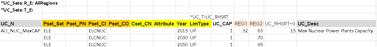
Figure 157. User Constraint to Impose a Maximum Capacity for Nuclear Power Plants
3.8.9. Results
The results for the electricity generation capacity (Figure 158) show the respective role of the new types of renewable power (biomass, hydro, wind and solar), the 2050 horizon, as well as the effects of the user constraint on nuclear capacity. Nuclear capacity remains constant for REG1 while it grows in REG2 up to the maximum bound in 2030, but not in 2050.
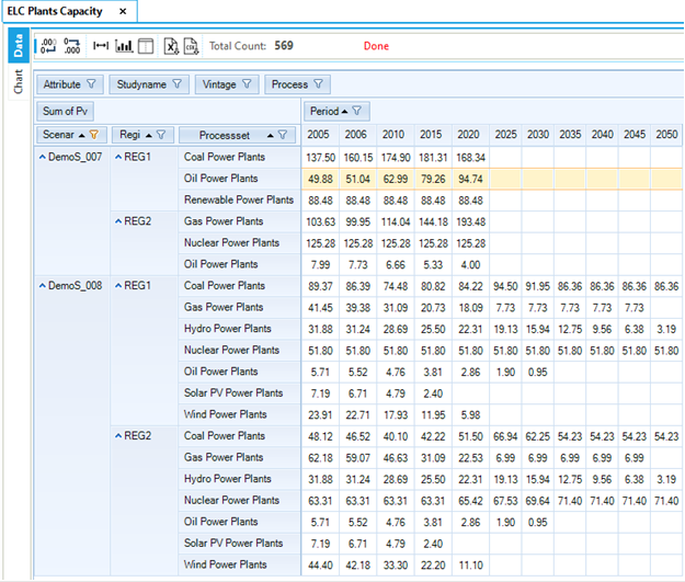
Figure 158. Results - Power Plant Capacity by Fuel Type in DemoS_008
The emissions by sector (in Mt) are presented in Figure 159 for both regions, where it is possible to see the contribution of each sector to reaching the reduction targets. In DemoS_008c, with a limit on the total emissions, the additional reductions are coming from the electricity sector (replacing coal-fired with gas-fired power plants), as well as from the residential and the commercial sectors (replacing solid fuels with renewable energies).
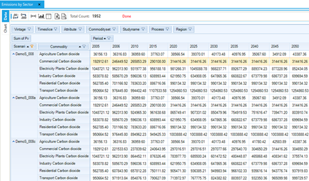
Figure 159. Emissions by Sector in DemoS_008
Objective-Function = 19,119,653 M euros (see the _SysCost table) with 9,068,703 M euros for REG1 and 10,050,950 M euros for REG2. These costs are again much higher to those computed in the previous step model DemoS_007 because of the expansion of the RES. The total cost is 4% higher with the emission limits for the electricity and the transportation sectors (19,358,261 M euros), and is only slightly reduced by the activation of the elastic demands (19,352,675 M euros). The additional user constraint on nuclear power increases the system cost by 11% (19,699,008 M euros).
3.9. DemoS_009 - SubRES sophistication (CHP, district heating) and Trans files
Description. At the ninth step, the model database is developed further by adding more SubRES with more complex processes. Because SubRES are used to add new processes in different sectors they can be considered as separate modules that can be included in model runs as part of the reference energy system or not. This approach is convenient when different individuals work in parallel on different sectors.
Objective. The objective is to give more examples of possible SubRES including more complex processes: one that introduces iron and steel production in the industrial sector, and one that introduces combined heat and power (CHP) processes, centralised heating plants, and heat exchanger + district heating network. Additional objectives include:
To show how to use the BY Trans file to move or add data and reduce the size of tables in the B-Y Templates. Here we specify the availability factor by time slice for existing wind and solar processes and add an interpolation rule for new hydro capacity (NCAP_BND).
To show how to use the transformation file associated with each SubRES to declare the availability or non-availability of each process in each region: new hydro power plants in this example.
To give an example of a scenario used to insert/update information in the B-Y Templates and SubRES: the demands and the retirement profile for the iron and steel processes.
To illustrate how to build a user constraint to limit the penetration of some processes, such as the district heating system between 2020 and 2050.
Attributes Introduced |
Files Updated |
|---|---|
PASTI |
VT_REG1/2_ELC_V09 |
CEH |
BY_Trans |
CHPR |
SubRES_NewTechs_Trans |
UC_CAP |
Files Created |
UC_COMPRD |
SubRES_New-IND |
UC_FLO |
SubRES_New-CHP-DH |
Scen_IND_NewRes |
|
Scen_UC_DH_MinProd |
Files. The ninth step model is built by:
modifying two B-Y Templates (VT_REG1_ELC_v09, VT_REG2_ELC_v09) to introduce past investment information;
using the BY Transformation file (BY_Trans) to insert base year information (availability factor by time slice for existing wind and solar plants and interpolation rules);
using a SubRES Transformation file (SubRES_NewTechs_Trans) to insert information for new processes (availability factor by time slice for new wind and solar plants) and to declare the availability or non-availability of each process in each region;
building two new SubRES (one with an iron & steel sector; one with CHP processes and district heating);
creating a scenario file to update information in the industrial sector;
creating a scenario file with a user constraint on the minimum penetration of district heating in the residential sector (Figure 160).
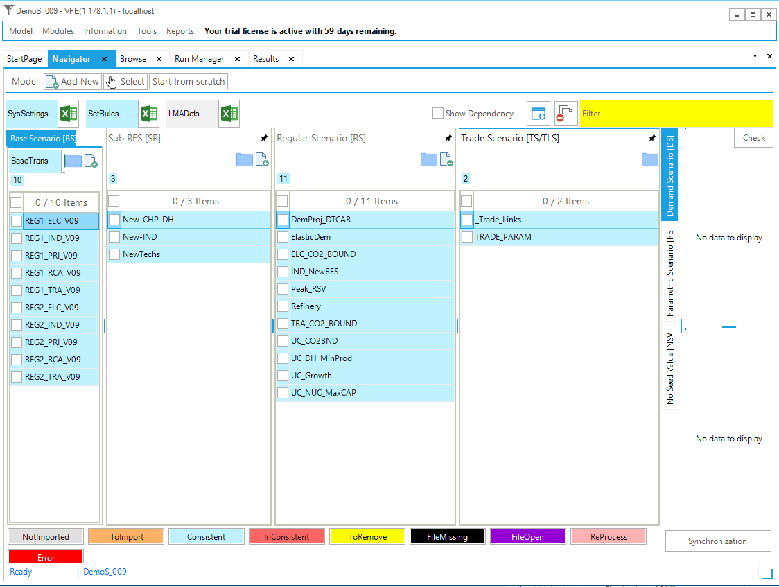
Figure 160. Templates Included in DemoS_009
3.9.1. B-Y Template VT_REG*_ELC_V09
The only B-Y Templates that are modified are the electricity ones (VT_REG1_ELC_V09 and VT_REG2_ELC_V09).
3.9.1.1. Con_ELC
The STOCK attribute for existing capacity can be replaced by another attribute (PASTI = past investments) to describe capacity installations that took place before the beginning of the model horizon (2005) and still exist during the modelling horizon. For any process, an arbitrary number of past investments may be specified to reflect the age structure in the existing capacity stock: the hydro power plants in this example (Figure 161). Each vintage of PASTI capacity will be constant until the end of its technical life, after which the capacity becomes zero in a single step. This allows a vintage-based retirement profile for the existing stock to be introduced into the model without the need to calculate and specify a STOCK in each future year.
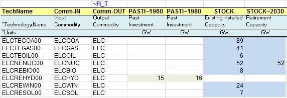
Figure 161. Past Investments That Occurred Before 2005
3.9.1.2. BY_Trans
The BY_Trans file works like a scenario file, except that the rule-based filters and the update/insert changes apply only to those process and commodities already existing in the B-Y templates. In this example (Figure 162), the file is used to insert new information: the availability factor (AF) by time slice (SD, SN, etc.) for existing wind and solar plants (ELCREWIN00 and ELCRESOL00).
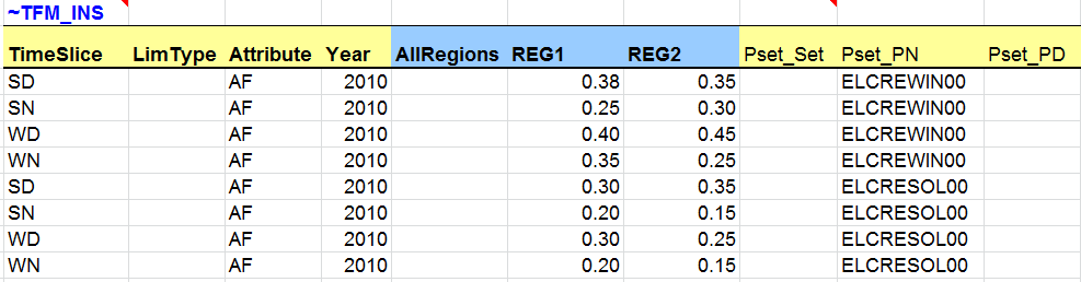
Figure 162. Transformation File to Insert New Attributes for Existing Processes
The transformation file is also used to insert a new interpolation rule (2 = interpolation, but extrapolation with EPS (epsilon, or effectively zero), which inserts EPS in every year if no bound value is declared in any year) to avoid the installation of new capacity (NCAP_BND) after the base year for the existing hydro power plants (ELCREHYD00). VEDA2.0 creates this entry by default for all technologies for which STOCK is declared. Since we have switched to using PASTI we need to declare it manually (Figure 163).

Figure 163. Transformation File to Insert a New Interpolation Rule
3.9.2. SubRES_NewTechs_Trans
Similarly to the BY_Trans file, a transformation file exists for each of the SubRES created. They are used to update/insert information for new processes and commodities declared in the corresponding SubRES and to declare the availability or non-availability of each process in each region. In this example, the transformation file of the SubRES_NewTechs is used to insert the availability factor for new wind and solar plants (ELCRNWIN01 and ELCRNSOL01) exactly as for the existing ones.
To assign the availability of processes to regions, a new ~TFM_AVA table is created (Figure 164). The first line says that all processes (Pset_PN=*) are available in all regions. The second line modifies this to say that the new hydro power plant is not available in REG1 (1=available; 0=non-available).
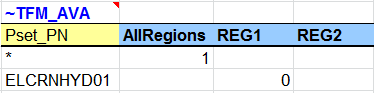
Figure 164. SubRES Transformation File to Set Process Availability
3.9.3. SubRES_New-IND
In the new SubRES_New-IND file, a simplified iron & steel sector is added to the model (Figure 165). This file includes two sheets (IND and PRI); sheet names need to start with the name of one of the model sectors.
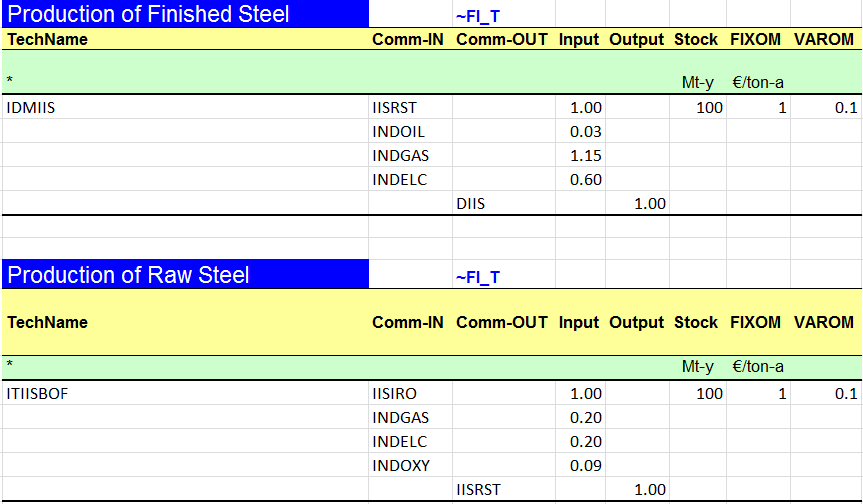
Figure 165. Iron & Steel Sector Processes
For policy analysis, it is useful to develop the most energy-intensive industrial sectors, such as iron & steel, in more detail, using a process-oriented approach rather than using generic processes capturing the energy mix. Here the demand is expressed in millions tons (Mt) of finished steel production, and a series of processes are modelled to represent the main steps of the transformation chain, from raw material extraction to the production of finished products (with capacity and activity units in Mt). The last process (IDMIIS) is described like a demand process, while the others are described as (upstream) processes in the chain. This means that they consume energy commodities and/or materials to produce new materials useful for the iron & steel chain production. The last process, which is a demand technology, finally consumes energy commodities and materials produced in the chain to satisfy the iron and steel demand (DIIS).
These processes use a mix of energy inputs and material inputs. These materials are declared as MAT commodities and tracked in Mt (Figure 166).
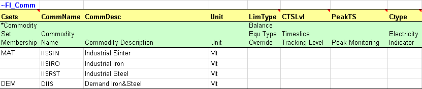
Figure 166. Energy and Material Input Commodities for the Iron & Steel Sector
3.9.4. SubRES_New-CHP-DH
This file includes two sheets (ELC_CHP and RCA), recalling that SubRES sheet names need to start with the name of one of the model sectors. The first sheet is used to add the combined heat and power (CHP) sector to the model (Figure 167). Cogeneration power plants, or combined heat and power plants (CHP), are plants that consume one or more commodities and produce two commodities, electricity (ELC) and heat (HET). The new CHP processes are characterized with additional attributes compared with conventional power plants.
The new processes do not have an existing installed capacity, but they are available in the database to be invested in. They are characterized with an efficiency (EFF), an annual availability factor (AFA), fixed and variable O&M costs (FIXOM, VAROM), a life time (LIFE), a capacity to activity factor (CAP2ACT in PJ/GW), and an investment cost (INVCOST), as well as the year in which they become available (START). Maximum input shares (Share-I~UP) are also specified for the dual input process ELCBNGAB01 consuming a maximum of 60% of biomass.
Two new attributes are introduced: the ratio of electricity lost to heat gained (CEH) as well as the ratio of heat produced to electricity produced (CHPR).
Two main types of cogeneration power plants can be distinguished according to the flexibility of the outputs: a back pressure process (ELCBNGAB01) and a condensing process (ELCCNGAS01).
Back pressure turbines are systems in which the ratio of the production of electricity and heat is fixed, so that the electricity generation is directly proportional to the steam produced. In a real system, a back pressure turbine is defined using the electrical efficiency, the thermal efficiency, and the load utilization. The CHPR attribute is then fixed (FX), so the production of electricity and heat is in a fixed proportion, but one could also use a (LO) CHPR for defining the back-pressure point, if so desired (to allow by-passing the turbine to produce more heat). CEH can be either 0 (or missing) or 1:
If it is 0 (or missing) as in this example, the activity represents the electricity generation and the capacity represents the electrical capacity;
If it is 1, the activity represents the total energy output and the capacity represents the total capacity (electricity + heat).
The condensing pass-out or extraction turbines do not have to produce heat, permitting electricity only to be generated, and permitting the amount of heat generated to be directly adjusted to the heat demand, while the electricity generation is reciprocally proportional to heat generation (electricity losses because of heat extraction). They are thus described differently:
Coefficient of electricity to heat, via attribute CEH such that: a) <= 1: electricity loss per unit of heat gained (moving from condensing to backpressure mode), indicating that activity is measured in terms of electricity, or b) >= 1: heat loss per unit of electricity gained (moving from backpressure to condensing mode), indicating that activity is measured in terms of total output (electricity plus heat).
Efficiencies, according to 1: a) are specified for the condensing point, or b) are specified for backpressure point.
Costs, according to 1 are specified based: a. according to condensing mode, or
b. on total electricity and heat output at backpressure point.
Ratio of heat produced to electricity produced (CHPR): Ratio of heat to power at backpressure point; at least a maximum value is required, but in addition also a minimum value may be specified.
See [Section 4.1]{.mark} of Part II of the TIMES documentation for more on CHP processes and their attributes.
The CHP processes are declared as CHP processes in the process declaration table with a time slice level of activity (DAYNITE). The heat (HET) is also declared as a new energy commodity in the commodity declaration table.
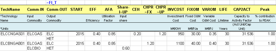
Figure 167. Combined Heat and Power Processes
The RCA sheet is used to add a district heating option to the model (Figure 168): a process is created as the district heating option (RSHNHET1) and a sector fuel process (FTE-RSDHET) is created to produce sector heat (RSDHET) from primary heat (HET).
They are characterized with an efficiency (EFF), an annual availability factor (AFA), fixed O&M costs (FIXOM), a life time (LIFE), a capacity to activity factor (CAP2ACT in PJ/GW), and an investment cost (INVCOST), as well as the year in which they become available (START).
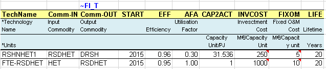
Figure 168. Demand for Heat and District Heating Options
3.9.5. Scenario files
3.9.5.1. Scen_IND_NewRES
A transformation table is used to update the base year industrial demand (DIDM1): the base year valued defined in the B-Y Templates are multiplied by 0.9 (Figure 169). This essentially reduces the DIDM1 demand that was used to model all industrial sector energy consumption by an amount roughly corresponding to that consumed by the new iron and steel sector. (Although note that we are not trying to replicate calibration to the energy balance precisely in this simple example.)
Another transformation table is used to define the demand value for the new iron and steel demand (DIIS), activating this sector when the SubRES is included in a model run, and to specify the retirement profile for the iron and steel processes (STOCK in 2050). (In this case the STOCK has been introduced in a SubRES template so VEDA2.0 will not create any interpolation rule to prohibit new investments.)


Figure 169. Update Existing Information and Insert New Information in the Industrial Sector
3.9.5.2. Scen_UC_DH_MinProd
A user constraint is built to specify the minimum district heating penetration requirement in specific years (2020 and 2050) with an interpolation/extrapolation rules between those years (rule 15=interpolation migrated at start, forward extrapolation) (Figure 170). The constraint says that the production of DRSH by processes that consume RSDHET (Pset_CI) must be the minimum (LimType=LO) percentage specified in each region/year combination of all production (table level declaration UC_COMPRD) of DRSH.

Figure 170. Minimum District Heating Penetration Using a User Constraint
3.9.6. Results
The model variant DemoS_009d is solved with the new iron & steel sector. Figure 171 shows the demand production (DIIS in Mt) from the finished steel production process (IDMIIS), consuming industrial steel (IISRST in Mt) and a mix of energy in PJ.
The model variant DemoS_009e is solved with the new district heating option. Figure 172 shows the contribution of district heat in meeting the demand for residential space heating in both regions together.
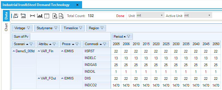
Figure 171. Results – Finished steel production in DemoS_009
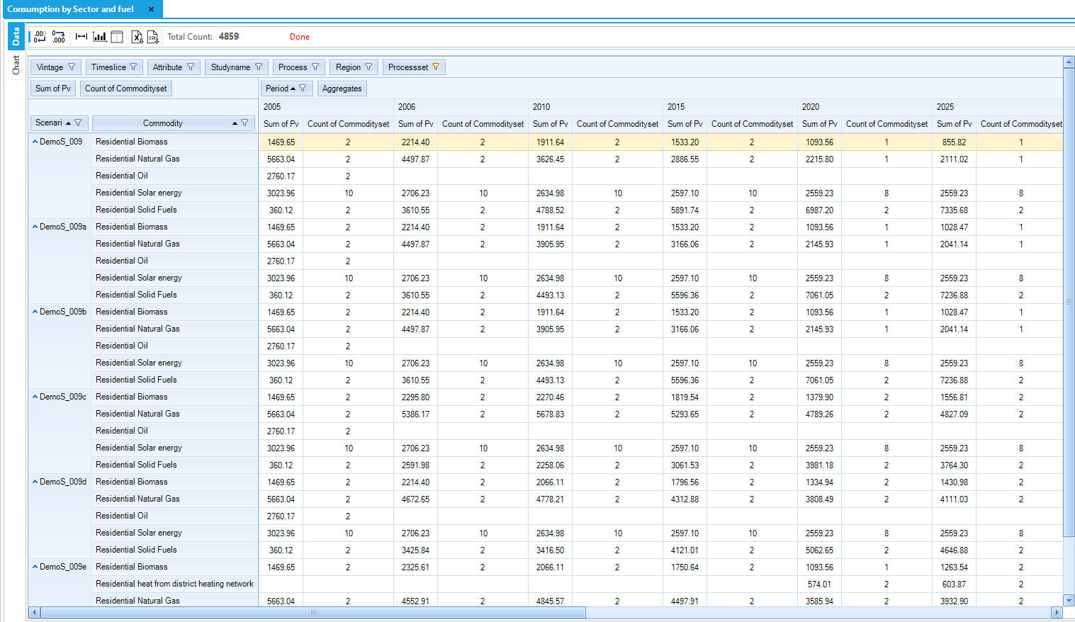
Figure 172. Residential Space Heating Fuel Use in DemoS_009
Objective-Function = 19,183,729 M euros (see the _SysCost table) with 9,084,193 M euros for REG1 and 10,099,536 M euros for REG2. These costs are similar to those computed with the previous step model DemoS_008. The total cost is 3% higher with the emission limits, growth rates, elastic demands, and the new iron and steel sector (19,721,879 M euros) and 5% with the new district heating option (20,187,883 M euros) and the new investment required to satisfy the minimum constraint on district heating penetration.
3.10. DemoS_010 - Demand projections and elastic demand
Description. At the tenth step, the model structure and database remain the same but energy service demands are projected using an internal VEDA2.0 routine.
Objective. The objective is to show how to prepare the files required to automatically project end-use demands for energy services using demand drivers along with sensitivity and calibration series.
Attributes Introduced |
Files Updated |
|---|---|
N.A. |
Scen_ElasticDem |
Files Created |
|
Dem_Alloc+Series |
|
ScenDem_DEM_Ref |
Files. The tenth step model is built:
by creating one file that allocates a demand driver to each end-use demand (Dem_Alloc+Series) and defines sensitivity and calibration series, and one file (ScenDem_DEM_Ref) that defines demand drivers;
by modifying the elastic demand scenarios to cover all end-use demands for energy services (Figure 173).
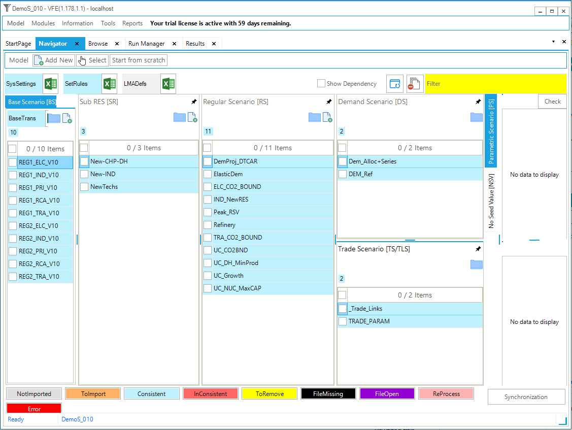
Figure 173. Templates Included in DemoS_010
3.10.1. Demand files
The Demand templates provide a means of preparing useful energy demand (or demand services) projections by means of using drivers and factors as discussed below.
3.10.1.1. ScenDem_DEM_Ref
The ~DRVR_Table table is used to declare a coherent set of driver growth rates (or indexes, with 2005=1) to drive all end-use demands in all regions (Figure 174). These drivers can be more general, such as macroeconomic indicators, as in this example (Gross Domestic Product (GDP), population (POP), industrial output demand (INDD)), or more specific, like vehicle-kilometres for energy service demands in the transportation sector, for instance. It is possible to build multiple files called ScenDem_<file name> with different drivers to generate, for example, a reference case along with low and high growth cases.
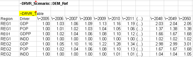
Figure 174. Drivers for End-use Demand Projections
3.10.1.2. Dem_Alloc+Series
The ~Series table is used to define sensitivity and calibration series (Figure 175). The sensitivity series represents the sensitivity of each end-use demand to one unit change in its driver. The calibration series can optionally be used to provide additional control over the resulting demand levels.
The growth rates of the various drivers are applied to the 2005 baseyear demands using the following formula:
The ~DRVR_Allocation table is used to allocate a particular driver to each end-use demand in each region (Figure 176). Only one such allocation file, always named Dem_Alloc+Series, may be built. That is, it is envisioned that in different scenarios, the projection of the driver for each demand may change (higher or lower population growth, for example), but the association of each demand with a particular driver will not change. (For example, DRSH is always driven by population growth with the same sensitivity.) Only one driver series may be associated with each demand. However, one may easily create a composite series if combining two drivers is desired. In this example, the demand DAOT will be projected using the driver GDP, adjusted with calibration and sensitivity series (Constant; =1 over the whole model horizon).
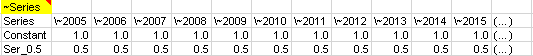
Figure 175. Sensitivity and Calibration Series for End-use Demand Projections
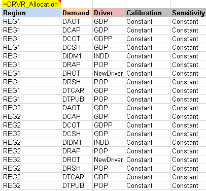
Figure 176. Allocation of Demand Drivers and Series for End-use Demand Projections
All the demands projected with the internal VEDA2.0 module can also be managed from the menu: Advanced Functions/Demand Master. Changes made within the Demand Master will be reflected in the templates. For more information on the Demand Master function, see http://support.kanors-emr.org/.
3.10.2. Results
The resulting demand projections in the reference case (DemoS_010) using the driver and series allocation presented above are shown in Figure 177.
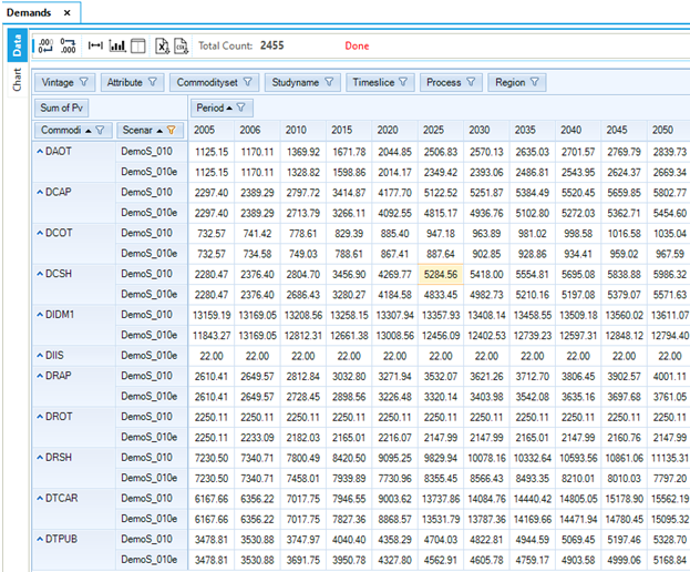
Figure 177. Demand Projection Results in DemoS_010
Objective-Function = 24,831,217 M euros (see the _SysCost table) with 10,869,234 M euros for REG1 and 13,961,983 M euros for REG2. The total cost is 7% higher with all model variants (26,475,198 M euros).
3.11. DemoS_011 – Sets Template
Description. At the eleventh step, the model structure and database remain the same, the main changes are in the SETS template and how to use it in scenario templates.
Objective. The objective is to show how to use user defined SETS (Sets-DemoModels) in a scenario file for model building and scenario analysis. As said above, it is possible to create sets of commodities and processes using the template Sets-<name>, that for the demo models is called Sets-DemoModels. These sets are generally used to build tables to view results in the Results module, but it is also possible to use these sets in VEDA templates. In this step there is an example of a user constraint on the minimum penetration of renewable power plants built using a user defined set of renewable processes.
Attributes Introduced |
Files Created |
|---|---|
N.A. |
Scen_BOUNDS-UC_WSETS |
Files. The eleventh step model is built:
by creating one scenario file that explains VEDA Sets specification and includes a user constraint..
3.11.1. Updating the Sets-DemoModels
The Sets-DemoModels template used in DemoS_011, includes the two sheets VEDA_Sets-Comm for commodities sets definition and VEDA_Sets-Proc for processes sets definition.
The commodity set rules are included in the model using the ~TFM_Csets, while the process sets throught ~TFM_Psets.
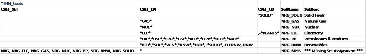
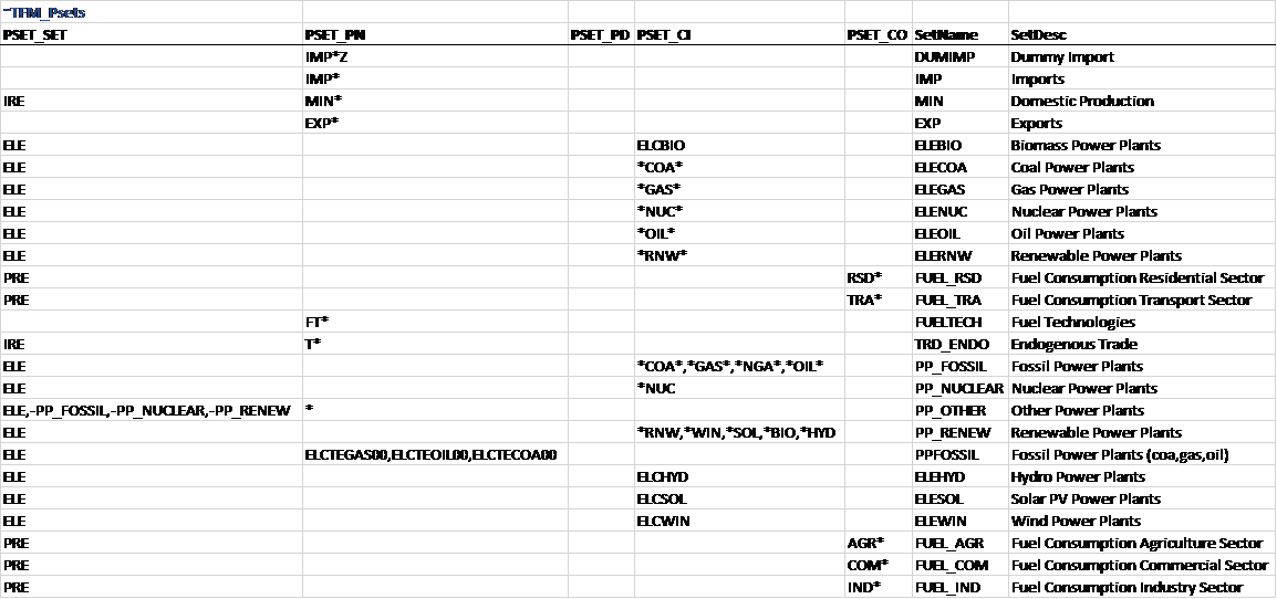
Figure 178. SETS Template in DemoS_010
The SET of interest for this model is the ones called PP_RENNEW (column SetName and described as Renewable Power plant in the column SetDesc), that is a process set built combining the information in the columns PSet_Set, to select the group of all processes that belongs to the TIMES set ELE, Pset_CI to identify the sub-group of ELE technologies that use in input commodities *RNW,*WIN,*SOL,*BIO and *HYD.
3.11.2. Scen_Bounds-UC-wSets
As an example, a user constraint is built using the process set PP_RENEW (column PSet_SET) that includes all renewable power plants: it specifies a minimum renewable penetration share of 10% in 2020 and 15%-20% in 2050, depending on the region, along with an interpolation/extrapolation rule (Figure 179).

Figure 179. User constraint on renewable power using a VEDA-BE set
3.11.3. Results
Figure 180 shows the impact of the new user constraint on the renewable share of total power generation. While the share of renewables is going to 0 without the user constraint in the previous reference case (DemoS_010), it reaches 18% across both regions in 2050 in the new reference case (DemoS_011), and 20% when including all additional constraints (limits on emissions, growth rates of cars, minimum penetration of district heating, etc.).
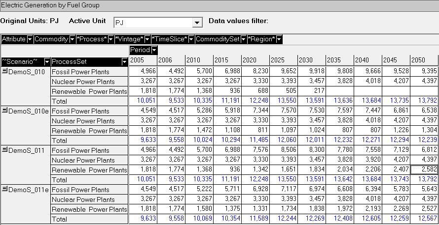
Figure 180. Generation in DemoS_010/011
Objective-Function = 24,867,969 M euros (see the _SysCost table) with 10,886,683 M euros for REG1 and 13,981,286 M euros for REG2. The total cost is 6% higher with all model variants (26,483,468 M euros).
3.12. DemoS_012 – More modelling techniques
Description. At the twelfth step, taxes and subsidies are added to the model database and a new modelling technique is introduced, namely the lumpy investment concept.
Objective. The objective is to show how to add taxes and subsidies for processes or commodities, such as a tax on diesel and total CO2 for all sectors and regions, as well as a subsidy on solar power plants in this example. Another objective is to show how to use the lumpy investment feature of TIMES through discrete capacity for the new nuclear power plants.
Attributes Introduced |
Files Updated |
|---|---|
N.A. |
VT_REG1/2_PRI_v12 |
SubRES_NewTechs |
|
Files Created |
|
Scen_TRADSL_Tax |
|
Scen_CO2_Tax |
|
Scen_Solar_Subsidies |
|
Scen_UC_CO2_Regions |
|
Scen_NUC_DiscInv |
Files. The twelfth step model is built by:
updating two B-Y Templates (VT_REG1_PRI_v12, VT_REG2_PRI_v12) to create an aggregated CO2 emission commodity;
updating the SubRES_NewTechs file to specify discrete investment options;
creating scenario files for introducing taxes, subsidies, and an emission constraint for all sectors and regions, as well as for discrete investments for nuclear power plants.
3.12.1. B-Y Template VT_REG*_Pri_V12
The only B-Y Templates that are modified are the primary energy ones (VT_REG1_PRI_V12 and VT_REG2_PRI_V12).
3.12.1.1. TOTCO2
A sheet is added with a ~COMAGG table is that is used to define an aggregated commodity (TOTCO2), including all sectoral CO2 emissions using multipliers of 1. This is equivalent to making TOTCO2 the sum of all sectoral CO2 emissions (Figure 181). It is possible to add more aggregated commodities and change multipliers. For instance, when there are different types of GHG emissions (CH4, N2O, etc.), an aggregated commodity can be created in CO2-equivalent to account for their respective global warming potential (CH4=36; N2O=298).
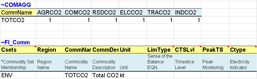
Figure 181. Aggregation of Emission Commodities
3.12.2. SubRES_NewTechs (ELC sheet)
The first step necessary to enable lumpy investments is to specify discrete investment options in the default process table, for new nuclear power plants in this example (ELCNNUC01), by changing the process set from ELC to ELC, DSCINV (Figure 182).
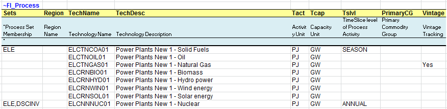
Figure 182. Discrete Investment Option for Nuclear Power Plants
3.12.3. Scenario files
3.12.3.1. Scen_NUC_DiscInv – lumpy investments
The second step necessary to enable lumpy investments is to specify allowable discrete capacity investments (NCAP_DISC) in specific years for new nuclear power plants (ELCNNUC01). In this example (Figure 183) the capacity installed for this process can be a module of 1 GW in 2015, while in 2033 the model can install 2 GW or 3 or 4 or 5 GW.
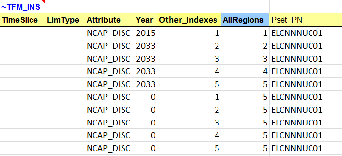
Figure 183. Discrete Capacity at Specific Years for Nuclear PowerPplants
In summary, the TIMES lumpy investment variant can be enabled following four steps:
Specify the SET DSCINV for the process for which lumpy investment is to be enabled (here new power plants (ELCNNUC01) in the ELC sheet of the SubRES_NewTechs file).
Build a scenario file with the discrete capacity modules to be allowed: capacities for the new power plants (ELCNNUC01) in the NUC_DSCINV sheet of the Scen_NUC_DiscInv scenario.
Before solving the model, it is necessary to enable the variant discrete investment in VEDA2.0. From the FE Case Manager, select the Control Panel button, check the box for Discrete Investment at the top right in the TIMES Extensions section (Figure 184), and click the OK button. Back in the FE Case Manager, the inscription DSC YES in the yellow section at the bottom of the window shows that the option is enabled.
In the Control Panel, set OPTCR (optimization criterion, or tolerance) to 0, in order to get a truly optimal solution. For example, if you leave OPTCR at its default value 0.1, in most models this will leave room for very different MIP solutions that would satisfy the optimality tolerance, and thus you could see lots of flip-flopping between model runs (even when using exactly the same scenario data).
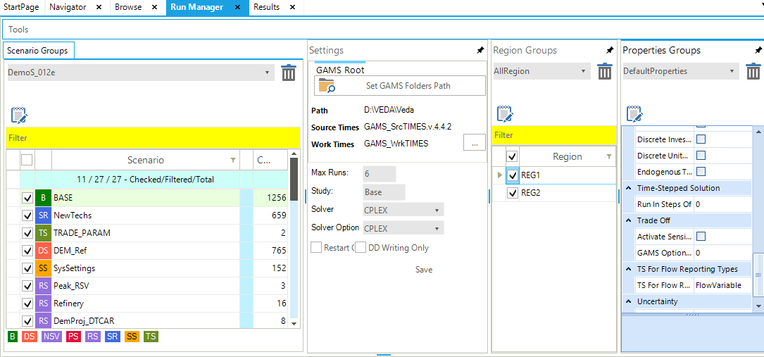
Figure 184. Enable the Variant Discrete Investment in VEDA2.0
3.12.3.2. Scen_TRADSL_Tax
This file is used to introduce a flow tax (FLO_TAX) on processes and commodities (input/output) (Figure 185). This is a new attribute that allows imposing an incremental cost of using/producing a commodity by a process (cost in Currency per unit of commodity produced or consumed). Here it is used to impose a flow tax on all the transportation processes (T*) consuming the diesel commodity (TRADSL) at specific years in each region.
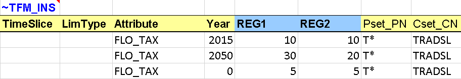
Figure 185. Flow Tax on Diesel
3.12.3.3. Scen_CO2_Tax
This file is used to introduce a tax on a net quantity of commodity (COM_TAXNET). Here we impose a tax on the new emission aggregated commodity (TOTCO2) created in B-Y Templates (VT_REG*_PRI_V12) at specific years (Figure 186).
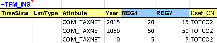
Figure 186. Tax on Net CO2 Emissions
3.12.3.4. Scen_Solar_Subsidies
This file is used to introduce a flow subsidy (FLO_SUB) on commodities (Figure 187). This is a new attribute that allows creating a credit for using/producing a commodity by a process (cost in Currency per unit of commodity produced or consumed). Here a flow subsidy on the electricity (ELC) commodity produced by all processes consuming the solar energy commodity (ELCSOL) is created with various values at specific years in each region.
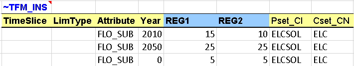
Figure 187. Subsidy on Electricity
3.12.3.5. Scen_UC_CO2_Regions
This file introduces a new user constraint that imposes limits on all CO2 emissions, summed over all regions and sector emissions. These upper bounds (or limits) are calculated as a percentage reduction target from the total CO2 emissions (TOTCO2 in kt) in a reference scenario for 2020 (10%) and 2050 (15%). It is necessary to run the step model without any limit on emissions first to get the reference emission trajectory (run DemoS_012) and to calculate the bounds as reduction from the reference emissions.
Comparing this scenario with Scen_UC_BND, the differences are the ~UC_Sets (using R_S: AllRegions rather than R_E: AllRegions) and the declaration (UC_RHSTS rather than UC_RHSRTS).
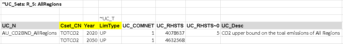
Figure 188. Cap Total CO2 Emission via User Constraint
3.12.4. Results
The impacts of the different taxes and subsidies, as well as the effects of the lumpy investment feature of TIMES through the discrete capacity requirement for the new nuclear power plants are shown in Error! Reference source not found. and Figure 190.
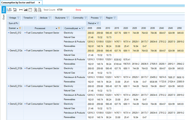
Figure 189. Final Energy Fuel Consumption in Transport
The impact on fuel consumption in the Transport section in are discussed below.
The tax on diesel consumption in the transportation sector (DemoS_012a) leads to a rapid decrease in refined products, reaching zero by 2025, to the benefit of renewable energies, which meet most of the demand by 2050.
The tax on total CO2 emissions (DemoS_012b) leads to an even more drastic decrease of refined products, reaching zero by 2010, to the benefit of renewable energies.
The limit on total CO2 emissions (DemoS_012d) does not have an impact on the transportation fuel mix but affects other parts of the whole energy system. The tax puts much higher pressure on the energy system than the limit.
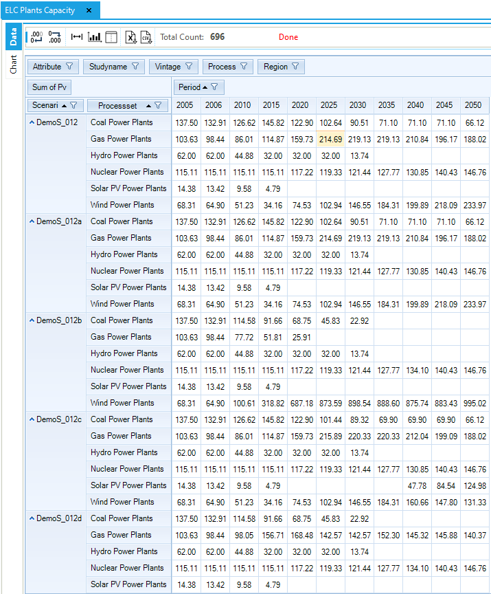
Figure 190. Electricity Power Plant Capacity in DemoS_012
The impact on the power sector in the various scenarios, as seen in Figure 190 shows are describing beow.
The tax on total CO2 emissions (DemoS_012b) has important impacts on the electricity sector as well, where most of the thermal generation capacity is replaced with wind power.
The subsidy on solar power (DemoS_012c) leads to a more diversified mix, as part of the wind power is replaced with solar power.
The declaration of discrete capacity for nuclear power plants (DemoS_012e) limits the nuclear growth, with only 1 GW of new capacity addition in 2020, 2025, 2030 and 10 GW in 2035 compared with 121 GW in the reference case (Figure 191). Note that to facilitate the comparing of the differences between the two scenarios the scenario was moved to the right of the power plant types.
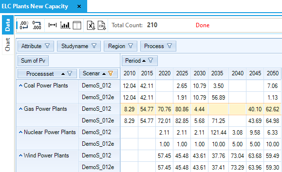
Figure 191. New Electric Plant Capacity Investments - DemoS_011/012 Comparison